Title here
Summary here
In Lesson 2 you turned every model call into a structured log record – one flat row per call with its prompt, response, tokens, latency, and cost. That row is perfect for answering “how many calls did we make, and what did they cost?” But it has a blind spot that shows up the moment Docent – our assistant for the Meridian serverless database docs – does more than one thing per request.
Here’s the blind spot. A single Docent request isn’t one model call. It retrieves the most relevant doc pages, then it generates an answer from them, and the agentic version searches the docs one or more times before it answers. When that whole request takes 1.2 seconds, a flat log line of the final model call can’t tell you where the 1.2 seconds went – was retrieval slow, or the model, or a second search you forgot was happening? And when a request fails, one row can’t tell you which step failed. You need to see the request as the sequence of steps it actually was.
That’s what distributed tracing gives you, and it’s the standard way every serious backend – LLM or not – follows a request through the systems it touches. This lesson brings it to Docent.
In this lesson, you will:
Span and a Tracer whose with tracer.span("generate") as s: records the span and wires up the tree, no external dependenciesdocent.request span contains a retrieve child and a generate child around a real claude-haiku-4-5 call, and read off where the time and tokens wentgenerate and tool spans appear in one multi-span traceTwo words carry the whole idea, so let’s pin them down precisely.
A span is one timed unit of work: a single retrieval, a single model call, a single tool call. Every span records five things:
retrieve, generate, tool.search_docs),A trace is one end-to-end request represented as the tree of spans that made it up. The parent-id pointers are what make it a tree: a top-level docent.request span is the root, and retrieve and generate hang off it as children because they carry its span id as their parent. Draw those spans on a shared time axis and you get a waterfall – each bar positioned by when it started and sized by how long it took – which is exactly the picture that tells you where a request spent its time.
Why is this the right shape for an LLM app specifically? Because an LLM request is inherently multi-step. Retrieval, then generation. Or search, read, search again, then answer. The cost and the latency and the failures are distributed across those steps, and a trace is the only view that keeps them attached to the step they belong to. A flat log throws that structure away; a trace preserves it.
Tracing is a standard, not a Claude-specific trick
Traces and spans come from distributed tracing (OpenTelemetry, and tools like Jaeger and Zipkin), where they follow a request as it hops across microservices. LLM-observability tools apply the exact same model to an LLM pipeline: a span per retrieval, per model call, per tool call. We build a tiny tracer by hand here so the mechanics are completely transparent – the same span tree, duration, and attributes you’d get from a production tracer, in about forty lines you can read end to end. Once you understand these forty lines, the vendor tools are just this with a nicer UI and a network exporter.
Let’s build it. We need two small classes and one convenience: a Span that holds the five fields above and computes its own duration, a Tracer that hands out spans and remembers who the parent is, and a print_trace helper to render the collected spans as an indented tree.
The one clever part is the parent tracking. We expose tracer.span(name) as a context manager, so you write with tracer.span("generate") as s: and the span is open for the duration of the with block. The tracer keeps a stack of currently-open spans: when a span opens it looks at the top of the stack to find its parent, then pushes itself; when it closes it records its end time and pops. Nesting with blocks therefore builds the tree automatically – whatever is open when you open a new span is its parent.
import time, itertools

class Span:
    """One timed unit of work in a trace."""
    def __init__(self, span_id, parent_id, name):
        self.span_id = span_id
        self.parent_id = parent_id
        self.name = name
        self.start = None
        self.end = None
        self.attributes = {}

    @property
    def duration_ms(self):
        return round((self.end - self.start) * 1000, 1)

class Tracer:
    """Collects spans into one trace. Use tracer.span(name) as a context manager."""
    def __init__(self, clock=time.perf_counter):
        self._clock = clock
        self._ids = itertools.count(1)
        self._stack = []      # currently-open spans (to find the parent)
        self.spans = []       # every finished span, in start order

    def span(self, name, **attributes):
        parent_id = self._stack[-1].span_id if self._stack else None
        s = Span(next(self._ids), parent_id, name)
        s.attributes.update(attributes)
        tracer = self

        class _Ctx:
            def __enter__(self):
                s.start = tracer._clock()
                tracer._stack.append(s)
                return s

            def __exit__(self, *exc):
                s.end = tracer._clock()
                tracer._stack.pop()
                tracer.spans.append(s)
                return False
        return _Ctx()

def print_trace(tracer):
    """Print the collected spans as an indented tree, each child under its parent."""
    by_parent = {}
    for s in tracer.spans:
        by_parent.setdefault(s.parent_id, []).append(s)

    def walk(parent_id, depth):
        for s in sorted(by_parent.get(parent_id, []), key=lambda x: x.start):
            pad = "  " * depth
            attrs = "  ".join(f"{k}={v}" for k, v in s.attributes.items())
            print(f"{pad}{s.name:<18} {s.duration_ms:>7} ms   {attrs}")
            walk(s.span_id, depth + 1)

    print(f"{'SPAN':<18} {'DURATION':>10}   ATTRIBUTES")
    print("-" * 62)
    walk(None, 0)
That’s the whole tracer – no dependencies, nothing Claude-specific. span() accepts attributes up front (tracer.span("retrieve", k=2)) and you can also set them on the returned span object inside the block (s.attributes["doc_ids"] = [...]) once you know the values.
Timing code is a place bugs love to hide, so before we point it at a live model we verify the mechanics – tree construction and duration arithmetic – on a fixed clock. Instead of the real wall clock, we feed the tracer a clock that returns pre-set tick values, so the durations are exact and identical on every run. This isolates the tracer’s logic from real-world jitter: if the numbers here ever change, it’s a bug in the tracer, not the network.
# A fake clock advancing on fixed, hand-set ticks. Each call returns the next
# value, so every duration is exact and reproducible -- no wall-clock jitter.
TICKS = iter([
    0.000,          # docent.request start
    0.010,          #   retrieve start
    0.034,          #   retrieve end   -> 24.0 ms
    0.040,          #   generate start
    0.930,          #   generate end   -> 890.0 ms
    0.935,          # docent.request end -> 935.0 ms
])
fixed_clock = lambda: next(TICKS)

tracer = Tracer(clock=fixed_clock)
with tracer.span("docent.request", question="rate limit code") as root:
    with tracer.span("retrieve", k=2) as r:
        r.attributes["doc_ids"] = ["errors", "ratelimits"]
    with tracer.span("generate", model="claude-haiku-4-5") as g:
        g.attributes["input_tokens"] = 214
        g.attributes["output_tokens"] = 38

print_trace(tracer)
SPAN DURATION ATTRIBUTES
--------------------------------------------------------------
docent.request 935.0 ms question=rate limit code
retrieve 24.0 ms k=2 doc_ids=['errors', 'ratelimits']
generate 890.0 ms model=claude-haiku-4-5 input_tokens=214 output_tokens=38Read the tree top to bottom. docent.request is the root (no parent), so it sits at the left margin; retrieve and generate are indented one level because each carries the root’s span id as its parent. The durations are the tick differences: retrieve ran from 0.010 to 0.034 (24 ms), generate from 0.040 to 0.930 (890 ms), and the root wraps both at 935 ms. Because the clock is fixed, running the block again prints byte-identical numbers:
SPAN                 DURATION   ATTRIBUTES
--------------------------------------------------------------
docent.request       935.0 ms   question=rate limit code
  retrieve              24.0 ms   k=2  doc_ids=['errors', 'ratelimits']
generate 890.0 ms model=claude-haiku-4-5 input_tokens=214 output_tokens=38The tracer’s logic is deterministic and correct. Now we swap the fake clock back for the real one and let a live request fill in real durations and real token counts.
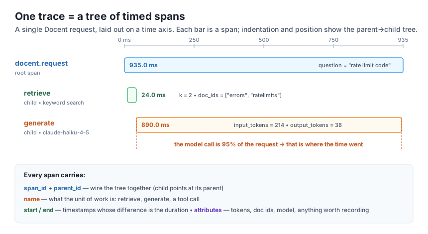
docent.request span (935 ms) contains a tiny retrieve child (24 ms) and a generate child (890 ms) drawn on a shared time axis. The waterfall makes the answer obvious at a glance: the model call is ~95% of the latency, so that's where any speed-up has to come from. Each span carries a span id, a parent id (to form the tree), a name, start/end times, and attributes like token counts and doc ids -- none of which a single flat log line preserves.Now the real thing. We take the minimal Docent – keyword retrieve plus a claude-haiku-4-5 generation – and wrap each step in a span. The root docent.request span opens first; inside it, a retrieve span records the doc ids it selected, and a generate span wraps the live model call and records the real input/output token counts pulled from the response’s usage. The with nesting does all the parent-wiring for us.
import time, itertools
import anthropic

client = anthropic.Anthropic()  # reads ANTHROPIC_API_KEY from the environment

# DOCS is the 8-page Meridian corpus defined earlier in the course (auth,
# ratelimits, plans, regions, errors, backups, sdks, deletion).
# Span / Tracer / print_trace are the classes defined above; print_trace here
# also truncates long attribute values so the waterfall stays readable.

def retrieve(question, docs, k=2):
    q = set(question.lower().split())
    scored = sorted(docs, key=lambda d: len(q & set((d["title"] + " " + d["text"]).lower().split())), reverse=True)
    return scored[:k]

def traced_docent(question, docs, tracer, model="claude-haiku-4-5"):
    with tracer.span("docent.request", question=question):
        with tracer.span("retrieve", k=2) as r:
            hits = retrieve(question, docs)
            r.attributes["doc_ids"] = [d["id"] for d in hits]
        ctx = "\n\n".join(f"[{d['id']}] {d['title']}\n{d['text']}" for d in hits)
        prompt = (f"Answer the question using ONLY the context. If the context does not contain the answer, say "
                  f"\"I don't have that in the docs.\" Be concise.\n\nContext:\n{ctx}\n\nQuestion: {question}")
        with tracer.span("generate", model=model) as g:
            msg = client.messages.create(model=model, max_tokens=200,
                                         messages=[{"role": "user", "content": prompt}])
            g.attributes["input_tokens"] = msg.usage.input_tokens
            g.attributes["output_tokens"] = msg.usage.output_tokens
        return msg.content[0].text

tracer = Tracer()  # real perf_counter clock
question = "What HTTP status code does Meridian return when you exceed the rate limit?"
answer = traced_docent(question, DOCS, tracer)

print("Question:", question)
print("Answer:  ", answer.replace("\n", " "))
print()
print_trace(tracer)
This is a live call, so the durations and the exact answer wording vary run to run – here is one real run (yours will differ by tens to hundreds of milliseconds, and the answer may be phrased differently):
Question: What HTTP status code does Meridian return when you exceed the rate limit?
Answer:   HTTP 429.

SPAN                 DURATION   ATTRIBUTES
------------------------------------------------------------------
docent.request      1209.3 ms   question=What HTTP status code does Meri...
  retrieve               0.1 ms   k=2  doc_ids=['errors', 'ratelimits']
  generate            1209.2 ms   model=claude-haiku-4-5  input_tokens=219  output_tokens=7
Now the trace earns its keep. Read straight down the durations: retrieve took 0.1 ms, generate took 1209.2 ms, and the root is 1209.3 ms – so essentially the entire request was the model call. That’s the kind of conclusion a flat log line of the final call literally cannot support, because it never recorded retrieval as a separate step to compare against. The attributes make it concrete too: retrieve shows exactly which pages it pulled (errors, ratelimits), and generate shows the real token split (219 in, 7 out). If this request had been slow, the trace tells you where to look before you write a single line of profiling code – and the answer is “the model, not retrieval,” so a keyword-retrieval tweak would be wasted effort here.
Attributes are where the debugging value lives
Durations tell you where the time went; attributes tell you why, and what. Recording doc_ids on the retrieve span means that when Docent gives a wrong answer, you can see whether the right page was even retrieved – a retrieval miss and a generation mistake look identical in the final answer but are completely different bugs. Recording input_tokens on the generate span means an unexpectedly slow or expensive request is one glance away from an explanation (“the context ballooned to 3,000 tokens”). Attach the few facts that would answer your next question before something breaks, because in production you can only debug what you captured – the same rule that opened this module.
The single-call trace has two children under one root. The picture gets more interesting – and tracing gets more essential – the moment a request makes several model calls. The agentic Docent from Module 6 does exactly that: it decides for itself to call the search_docs tool, gets results back, and then makes a second model call to write the answer. That’s two generations and a tool call in one request, and a flat log would scatter them across three unrelated rows. A trace keeps them together as one tree.
We instrument it with the same tracer – no new machinery. Each turn of the agent loop opens a generate span (recording tokens and the stop_reason), and each tool call opens a tool.search_docs span (recording the query and the doc ids it returned):
import time, itertools, json
import anthropic

client = anthropic.Anthropic()  # reads ANTHROPIC_API_KEY from the environment

SEARCH_TOOL = [{
    "name": "search_docs",
    "description": "Search the Meridian documentation and return matching pages. Call this before answering.",
    "input_schema": {
        "type": "object",
        "properties": {"query": {"type": "string", "description": "search query"}},
        "required": ["query"],
    },
}]

def search_docs(query, docs, k=2):
    q = set(query.lower().split())
    scored = sorted(docs, key=lambda d: len(q & set((d["title"] + " " + d["text"]).lower().split())), reverse=True)
    hits = scored[:k]
    return [{"id": d["id"], "title": d["title"], "text": d["text"]} for d in hits]

def traced_agentic_docent(question, docs, tracer, model="claude-haiku-4-5", max_steps=4):
    system = ("You are Docent, a Meridian docs assistant. Use the search_docs tool to find relevant pages, "
              "then answer ONLY from what it returns. If the docs don't contain the answer, say "
              "\"I don't have that in the docs.\"")
    messages = [{"role": "user", "content": question}]
    with tracer.span("docent.request", question=question):
        for _ in range(max_steps):
            with tracer.span("generate", model=model) as g:
                resp = client.messages.create(model=model, max_tokens=400, system=system,
                                               tools=SEARCH_TOOL, messages=messages)
                g.attributes["input_tokens"] = resp.usage.input_tokens
                g.attributes["output_tokens"] = resp.usage.output_tokens
                g.attributes["stop"] = resp.stop_reason
            if resp.stop_reason == "tool_use":
                messages.append({"role": "assistant", "content": resp.content})
                tool_results = []
                for block in resp.content:
                    if block.type == "tool_use":
                        with tracer.span("tool.search_docs", query=block.input["query"]) as t:
                            hits = search_docs(block.input["query"], docs)
                            t.attributes["doc_ids"] = [h["id"] for h in hits]
                        tool_results.append({"type": "tool_result", "tool_use_id": block.id,
                                             "content": json.dumps(hits)})
                messages.append({"role": "user", "content": tool_results})
            else:
                text = "".join(b.text for b in resp.content if b.type == "text")
                return text

tracer = Tracer()
question = "What HTTP status code does Meridian return when you exceed the rate limit?"
answer = traced_agentic_docent(question, DOCS, tracer)
print("Answer:", answer.replace("\n", " "))
print()
print_trace(tracer)
One real run (again, live – durations and phrasing will vary, though the shape is stable: generate, tool call, generate):
Answer: Meridian returns HTTP status code **429** when you exceed the rate limit. This response includes a `Retry-After` header that indicates the number of seconds you should wait before making another request.

SPAN               DURATION   ATTRIBUTES
--------------------------------------------------------------
docent.request    3775.4 ms   question=What HTTP status code does Meri...
  generate          2366.6 ms   model=claude-haiku-4-5  input_tokens=644  output_tokens=58  stop=tool_use
  tool.search_docs     0.1 ms   query=rate limit HTTP status code  doc_ids=['errors', 'ratelimits']
  generate          1408.7 ms   model=claude-haiku-4-5  input_tokens=894  output_tokens=45  stop=end_turn
Now the trace shows the request’s real anatomy: two model calls with a tool call between them, and the durations attached to each. The first generate (2367 ms, stop=tool_use) is the model deciding to search; the tool.search_docs span shows the query it chose and that it retrieved errors and ratelimits; the second generate (1409 ms, stop=end_turn) writes the final answer from those results. Add the two model calls and you see why the agentic request took 3.8 seconds versus the single-call version’s 1.2 – it paid for two generations, and the trace hands you that breakdown for free. The input_tokens climbing from 644 to 894 between the two calls even shows the tool results being folded into the context. This is the whole argument for tracing an LLM app: a single flat log line could never have told you any of that.
error attribute when a span’s work raisesRight now a span that throws mid-block still gets recorded (the __exit__ runs), but nothing marks it as failed. Modify the tracer’s __exit__ so that when the block exits with an exception, it sets s.attributes["error"] to the exception’s string and still records the span. Then wrap a generate span around a call that deliberately raises (e.g. a bad model id) and confirm the failed span appears in the trace with its error attribute and a real duration.
Hint
__exit__ receives (exc_type, exc_value, exc_tb). Change its signature to capture them and add if exc_type is not None: s.attributes["error"] = str(exc_value) before you append the span. Keep return False so the exception still propagates – a tracer should observe failures, not swallow them. The span’s end time is set regardless, so a failed call still shows how long it ran before dying, which is often exactly what you want to know (did it time out, or fail instantly?).
A span’s total duration includes its children, so the root always looks like the slowest thing – that’s not useful for finding a bottleneck. Write self_time(tracer) that returns, for each span, its own time: its duration minus the summed durations of its direct children. Run it on the single-call live trace and confirm that docent.request’s self-time is tiny (it does almost nothing itself) while generate’s self-time equals its full duration (it has no children).
Hint
Build a children map like print_trace does (by_parent), then for each span subtract sum(c.duration_ms for c in children_of[span.span_id]) from its own duration_ms. Self-time is what production trace UIs use to color the actually expensive span: on the single-call trace, generate will hold essentially all the self-time, which correctly says “optimize the model call, not the wrapper.” On the agentic trace, sum the self-time of the two generate spans to see the true model cost of the request.
trace_id and export it as JSONA real tracer tags every span in one request with the same trace_id so you can store spans from thousands of requests together and still reassemble each tree. Add a trace_id (e.g. a short random hex string) to the Tracer, stamp it onto every span, and write export(tracer) that returns a list of plain dicts – trace_id, span_id, parent_id, name, duration_ms, attributes – ready to be written as JSON lines. Verify the exported list round-trips: rebuild the indented tree from the dicts alone.
Hint
import uuid; trace_id = uuid.uuid4().hex[:8] in the tracer’s __init__, then set s.trace_id = self._trace_id when you create each span. export is a list comprehension over tracer.spans. This is precisely the boundary between our teaching tracer and a production one: production spans are just dicts like these, shipped over the network to a backend that groups them by trace_id and draws the waterfall. Reconstructing the tree from the dicts alone proves the parent_id pointers – not any in-memory object references – are what actually hold the trace together.
A trace is one end-to-end request modeled as a tree of spans, where each span is a timed unit of work carrying a span id, a parent span id (which wires the tree), a name, start/end times whose difference is its duration, and attributes like token counts and doc ids. For an LLM app this is the right shape because a request is inherently multi-step – retrieval plus one or more model calls plus tools – and a single flat log line can’t tell you where the time and tokens went or which step failed, while a trace keeps every fact attached to the step it belongs to. You built a minimal tracer in pure Python: a Span/Tracer pair whose with tracer.span("generate") as s: context manager records the span and uses a stack of open spans to wire up parents automatically, plus a print_trace that renders the tree indented. You proved the tree-and-duration mechanics reproducible by running them on a fixed clock (935 ms root, 24 ms retrieve, 890 ms generate, byte-identical twice), then instrumented a live Docent request and read the real breakdown straight off the trace – retrieve 0.1 ms versus a claude-haiku-4-5 generate of ~1209 ms, i.e. the model call was essentially the whole request. Finally you traced the agentic Docent and got a genuine multi-span trace – two generate spans around a tool.search_docs span – that explained why the agentic request took ~3.8 s where the single call took ~1.2 s.
with blocks set it automatically.When Docent is live and a request is slow or wrong at 2 a.m., a flat log of the final model call leaves you guessing which of retrieval, the first generation, a tool call, or the second generation was to blame – and guessing is expensive. A trace removes the guess: the waterfall shows you the slow span directly, and the attributes on that span (which pages were retrieved, how many tokens went in, what the stop reason was) usually show you why before you attach a debugger. That’s the difference between “the request took 4 seconds” and “the second generation took 2.4 seconds on a 3,000-token context because retrieval pulled the wrong pages” – the first is a shrug, the second is a fix. The tracer you built is deliberately tiny, but it is the same span tree, duration, and attribute model that OpenTelemetry and every LLM-observability vendor use; the production tools add a UI and a network exporter, not a new idea. With logging (Lesson 2) and tracing (this lesson) in place, every Docent request now leaves behind a record you can actually read. Next you’ll put hard numbers on the two things those traces surface most – cost and latency – including the percentiles that reveal the slow tail an average hides.
You can now follow a single Docent request through the steps it actually took. You learned the core model – a trace is one request, a tree of timed spans, each with a span id, a parent id, a name, start/end times, and attributes – and built a minimal tracer in pure Python whose with tracer.span(...) context manager records each span and wires the parent tree from a stack of open spans, with no external dependencies. You proved the tree-and-duration mechanics reproducible on a fixed clock, then instrumented a live claude-haiku-4-5 Docent request and read the breakdown straight off the trace: retrieval was 0.1 ms and the model call was essentially the entire ~1.2 s, a conclusion a flat log line structurally cannot support. Then you extended the same tracer to the agentic Docent and captured a real multi-span trace – two generations around a tool call – that explained the request’s full ~3.8 s cost. That is exactly the model production observability tools use; you built it by hand so nothing about it is a black box. In Lesson 4 you’ll take the durations and token counts these spans capture and turn them into rigorous cost, latency, and token accounting – averages, and the p50/p95 percentiles that expose the slow, expensive tail an average quietly hides.
Keep DATATWEETS free. Help fund practical data, AI, and engineering lessons for learners worldwide.
