Lesson 4 - Cost, Latency & Token Accounting

Welcome to Cost, Latency & Token Accounting#

The last two lessons taught you to capture what Docent – our assistant for the Meridian serverless database docs – does in production: structured logs of every model call, and traces that follow a request through retrieval and generation. Those tell you what happened. This lesson turns the same captured data into the three numbers that decide whether Docent is viable at all: tokens, cost, and latency.

Here’s why they belong together. Every Docent call spends tokens; tokens drive the bill and the response time; and response time is what a user actually experiences while waiting for an answer. A version of Docent that’s brilliant but costs 10 dollars per question, or that answers in 200 milliseconds for most users but hangs for eight seconds for one in twenty, doesn’t ship – no matter how well it scores on the eval sets from earlier modules. Operational accounting is the check that quality evaluation can’t do for you.

The subtlety is in how you report each one. Tokens split into input and output, and output usually costs several times more per token – so a metric that lumps them together misleads you about cost. Cost is only meaningful if you compute it from real token counts against a real price. And latency is the trap: report the mean and you’ll cheerfully hide the slow tail that generates every angry support ticket. The fix is percentiles. We’ll build all three from live Docent runs and assemble them into one operational report.

In this lesson, you will:

• Read real input_tokens and output_tokens off msg.usage and see why the split matters for cost
• Compute per-request and total cost from real token counts and a clearly-labeled illustrative claude-haiku-4-5 price
• Implement latency percentiles (p50/p95/p99) and see why the mean hides the slow tail that users feel
• Run Docent live over a small batch, capturing real tokens and latency per request
• Assemble a single aggregate operational report – total/mean tokens, total cost, cost per 1000 requests, mean/p50/p95 latency – and prove the aggregation math is reproducible

Tokens: input vs output, straight from usage#

Every response from the API carries a usage object with the exact token counts the call was billed on – you don’t estimate them, you read them. There are two that matter here: input tokens (everything you sent – the prompt, which for Docent means the retrieved context plus the question) and output tokens (everything the model generated – the answer). Keep them separate, because they’re priced separately and they behave differently: input tokens are large and fairly fixed per request (Docent’s prompt is dominated by the two retrieved doc pages), while output tokens are small but, per token, the expensive ones.

Here’s Docent, unchanged from the course’s canonical version except that we return the two token counts alongside the answer so we can account for them. Run it once and read the usage off a real call:

import warnings
warnings.filterwarnings("ignore")
import anthropic

client = anthropic.Anthropic()  # reads ANTHROPIC_API_KEY from the environment

DOCS = [
    {"id": "auth", "title": "Authentication",
     "text": "Meridian authenticates every request with an API key sent in the Authorization header as a bearer token. "
             "Create keys in the dashboard under Settings > API Keys. Keys are either test or live mode; test keys only "
             "touch sandbox data. A key is shown once at creation and cannot be recovered, only rotated."},
    {"id": "ratelimits", "title": "Rate Limits",
     "text": "The Free plan allows 60 requests per minute. The Pro plan allows 600 requests per minute. Exceeding the "
             "limit returns HTTP 429 with a Retry-After header giving the seconds to wait. Rate limits are applied per "
             "API key, not per account."},
    {"id": "plans", "title": "Plans and Pricing",
     "text": "Meridian has three plans. Free costs 0 dollars per month and includes 1 GB of storage. Pro costs 25 dollars "
             "per month and includes 50 GB of storage. Scale costs 199 dollars per month and includes 500 GB of storage. "
             "All plans include unlimited read replicas."},
    {"id": "regions", "title": "Regions",
     "text": "Databases can be created in three regions: us-east, eu-west, and ap-south. The region is fixed at creation "
             "time and cannot be changed later; to move data to another region you must export and re-import into a new "
             "database. Cross-region read replicas are available on the Scale plan only."},
    {"id": "errors", "title": "Error Codes",
     "text": "Meridian uses standard HTTP status codes. 400 means a malformed request, 401 means a missing or invalid API "
             "key, 403 means the key is valid but lacks permission, 404 means the resource does not exist, and 429 means "
             "the rate limit was exceeded. 5xx codes indicate a server-side error and should be retried with backoff."},
    {"id": "backups", "title": "Backups",
     "text": "Automatic daily backups are retained for 7 days on the Free plan, 30 days on Pro, and 90 days on Scale. "
             "Backups run at 03:00 UTC. Point-in-time recovery to any second in the retention window is available on the "
             "Scale plan. Restoring a backup creates a new database and never overwrites the original."},
    {"id": "sdks", "title": "SDKs",
     "text": "Official SDKs are available for Python, JavaScript, and Go. Install the Python SDK with 'pip install meridian'. "
             "The SDK reads the MERIDIAN_API_KEY environment variable by default. All SDKs retry idempotent requests up to "
             "3 times on 5xx errors with exponential backoff."},
    {"id": "deletion", "title": "Deleting Data",
     "text": "Deleting a database is immediate and irreversible once the 24-hour grace period ends. During the grace period "
             "the database is soft-deleted and can be restored from the dashboard. After 24 hours the data and its backups "
             "are permanently purged. Deletion requires a live-mode key with admin permission."},
]

def retrieve(question, docs, k=2):
    q = set(question.lower().split())
    scored = sorted(docs, key=lambda d: len(q & set((d["title"] + " " + d["text"]).lower().split())), reverse=True)
    return scored[:k]

def docent_answer(question, docs, model="claude-haiku-4-5"):
    """Return (answer_text, input_tokens, output_tokens) -- the token counts come
    straight from the API's usage object, not an estimate."""
    ctx = "\n\n".join(f"[{d['id']}] {d['title']}\n{d['text']}" for d in retrieve(question, docs))
    prompt = (f"Answer the question using ONLY the context. If the context does not contain the answer, say "
              f"\"I don't have that in the docs.\" Be concise.\n\nContext:\n{ctx}\n\nQuestion: {question}")
    msg = client.messages.create(model=model, max_tokens=200,
                                 messages=[{"role": "user", "content": prompt}])
    return msg.content[0].text, msg.usage.input_tokens, msg.usage.output_tokens

answer, in_tok, out_tok = docent_answer("How much does the Pro plan cost per month?", DOCS)
print("answer       :", answer.strip())
print("input_tokens :", in_tok)
print("output_tokens:", out_tok)
print("total_tokens :", in_tok + out_tok)

answer       : The Pro plan costs $25 per month.
input_tokens : 199
output_tokens: 13
total_tokens : 212

Look at the shape of that: 199 input tokens, 13 output tokens. The prompt is fifteen times larger than the answer, which is typical for a retrieval assistant – you pay to send the model two doc pages so it can write one short sentence. This is a real live call, so if you run it your exact counts may differ by a token or two as the model words the answer slightly differently; the shape (a large input, a tiny output) will hold. That shape is exactly why the next step – pricing – can’t just multiply total tokens by one number.

Cost: real token counts times a real price#

Cost is mechanical once you have the token counts. The catch is that input and output tokens have different prices, and output is the pricier side per token, so you price the two streams separately and add them:

Prices are quoted per million tokens. For this lesson we’ll use an illustrative price for claude-haiku-4-5 of 1.00 dollars per million input tokens and 5.00 dollars per million output tokens.

Apply the formula to the real counts from the call above (199 input, 13 output):

# ILLUSTRATIVE prices for claude-haiku-4-5, dollars per MILLION tokens.
# Prices change; treat as illustrative, not a live quote.
PRICE_IN_PER_M = 1.00
PRICE_OUT_PER_M = 5.00

def request_cost(in_tok, out_tok):
    return in_tok / 1_000_000 * PRICE_IN_PER_M + out_tok / 1_000_000 * PRICE_OUT_PER_M

in_tok, out_tok = 199, 13  # real usage from the call above
print(f"input : {in_tok:>3} tok @ ${PRICE_IN_PER_M:.2f}/M  -> ${in_tok / 1_000_000 * PRICE_IN_PER_M:.6f}")
print(f"output: {out_tok:>3} tok @ ${PRICE_OUT_PER_M:.2f}/M  -> ${out_tok / 1_000_000 * PRICE_OUT_PER_M:.6f}")
print(f"cost per request   : ${request_cost(in_tok, out_tok):.6f}")
print(f"cost per 1000 reqs : ${request_cost(in_tok, out_tok) * 1000:.4f}")

input : 199 tok @ $1.00/M  -> $0.000199
output:  13 tok @ $5.00/M  -> $0.000065
cost per request   : $0.000264
cost per 1000 reqs : $0.2640

A single Docent answer costs about a quarter of one-thousandth of a dollar. That feels like nothing – and per request it is. But operational cost is a per-request number multiplied by request volume, so the unit to reason in is “per 1000 requests”: at this rate, 1000 Docent questions cost about 26 cents. Now the number is legible: a support portal fielding a hundred thousand questions a day is spending real money, and a prompt change that doubles the retrieved context (doubling input tokens) is a line item you can see. This block is pure arithmetic on fixed inputs, so it’s perfectly reproducible – run it twice and you get $0.000264 both times, unlike the live call that produced the token counts.

Latency: report percentiles, not the mean#

Cost you can compute from tokens; latency you have to measure, because it depends on the network, the model’s load, and how much it generated. The measurement itself is easy – wall-clock time around the call with time.time(). The hard part is reporting it honestly.

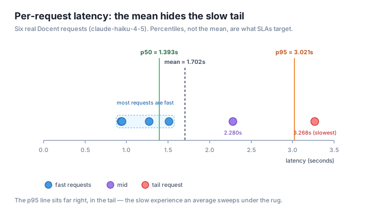
The instinct is to report the average. Resist it. Consider six real Docent latencies: five of them land between 0.9 and 1.5 seconds, and one takes 3.3 seconds. The mean is about 1.7 seconds – a number that describes none of the actual requests: it’s slower than the five fast ones and faster than the slow one. And it completely buries the 3.3-second request, which is the one whose user was staring at a spinner. That slow request isn’t noise; in production it’s a whole slice of your traffic, and it’s the slice that files tickets and churns.

The honest report is percentiles. The p50 (the median) is the value half your requests come in under; p95 is the value 95% come in under – so 1 request in 20 is slower than p95; p99 is the tail’s tail. SLAs are written in these terms (“p95 under 2 seconds”) precisely because they describe the experience of your slowest users, not a mythical average one. Here’s a percentile implementation and the split it produces on those six real latencies:

# Real per-request latencies (seconds) captured from six live Docent calls.
LAT = [2.280, 1.513, 3.268, 0.931, 0.944, 1.274]

def percentile(values, p):
    """The p-th percentile (0-100) via linear interpolation between ranks."""
    s = sorted(values)
    if len(s) == 1:
        return s[0]
    rank = (p / 100) * (len(s) - 1)   # fractional position in the sorted list
    lo = int(rank)
    frac = rank - lo
    if lo + 1 >= len(s):
        return s[lo]
    return s[lo] + frac * (s[lo + 1] - s[lo])   # interpolate between neighbors

mean = sum(LAT) / len(LAT)
print(f"sorted latencies : {sorted(LAT)}")
print(f"mean : {mean:.3f}s")
print(f"p50  : {percentile(LAT, 50):.3f}s")
print(f"p95  : {percentile(LAT, 95):.3f}s")
print(f"p99  : {percentile(LAT, 99):.3f}s")

sorted latencies : [0.931, 0.944, 1.274, 1.513, 2.28, 3.268]
mean : 1.702s
p50  : 1.393s
p95  : 3.021s
p99  : 3.219s

Read the gap between the numbers. The p50 is 1.393s – that’s the typical Docent request, and it sits right inside the fast cluster where most calls actually live. The p95 is 3.021s, more than double the median: it has climbed out to where the slow requests are, and it’s the number that honestly answers “how bad is it for the users having a bad time?”. The mean, at 1.702s, splits the difference and tells you about neither group. The percentile function is deterministic – it sorts and interpolates a fixed list with no model in the loop – so it returns the identical values every run, which is exactly what you want from a metric you’ll compute over millions of production requests.

Putting it together: an aggregate operational report#

Individually these metrics are useful; together they’re a dashboard. The workflow is: run a batch of Docent requests, capture the real tokens and real latency for each, then aggregate. First the live capture – six Meridian questions through Docent, timing each call and recording its usage:

import time

QUESTIONS = [
    "What HTTP status code does Meridian return when you exceed the rate limit?",
    "How many requests per minute does the Pro plan allow?",
    "How much does the Pro plan cost per month?",
    "How long are backups retained on the Scale plan?",
    "What does a 401 error mean?",
    "What environment variable does the Python SDK read for the API key?",
]

records = []  # each record: {"in": input_tokens, "out": output_tokens, "latency": seconds}
print("Live capture over Docent (claude-haiku-4-5)")
print("=" * 70)
for q in QUESTIONS:
    t0 = time.time()
    answer, in_tok, out_tok = docent_answer(q, DOCS)
    latency = time.time() - t0                       # real wall-clock time for this call
    records.append({"in": in_tok, "out": out_tok, "latency": latency})
    print(f"in={in_tok:>3}  out={out_tok:>2}  latency={latency:.3f}s  | {answer.strip()[:52]}")

Live capture over Docent (claude-haiku-4-5)
======================================================================
in=219  out=16  latency=2.280s  | HTTP 429 is returned when the rate limit is exceeded
in=200  out=14  latency=1.513s  | The Pro plan allows 600 requests per minute.
in=199  out=13  latency=3.268s  | The Pro plan costs $25 per month.
in=220  out=18  latency=0.931s  | Backups are retained for 90 days on the Scale plan.
in=213  out=16  latency=0.944s  | A 401 error means a missing or invalid API key.
in=226  out=22  latency=1.274s  | The Python SDK reads the `MERIDIAN_API_KEY` enviro

That’s a real run. The token counts are stable request to request (input hovers around 200-226, output around 13-22 – retrieval prompts are consistent), but latency is genuinely variable: the same “Pro plan cost” question that took 3.268s here might take under a second on your machine or on a re-run, because latency depends on network and server load, not just on the work. That’s the whole reason we report a distribution of latency and a point estimate of tokens.

Now aggregate. To keep the report reproducible, we compute it over the fixed list of records captured above – the aggregation is pure math on fixed inputs, so it must return identical numbers every time, even though the live capture that fed it will vary:

# Frozen from the live capture above: (input_tokens, output_tokens, latency_seconds).
RECORDS = [
    {"in": 219, "out": 16, "latency": 2.280},
    {"in": 200, "out": 14, "latency": 1.513},
    {"in": 199, "out": 13, "latency": 3.268},
    {"in": 220, "out": 18, "latency": 0.931},
    {"in": 213, "out": 16, "latency": 0.944},
    {"in": 226, "out": 22, "latency": 1.274},
]

def operational_report(records):
    n = len(records)
    total_in = sum(r["in"] for r in records)
    total_out = sum(r["out"] for r in records)
    total_cost = sum(request_cost(r["in"], r["out"]) for r in records)
    lat = [r["latency"] for r in records]
    return {
        "requests": n,
        "total_input_tokens": total_in,
        "total_output_tokens": total_out,
        "total_tokens": total_in + total_out,
        "mean_tokens_per_request": (total_in + total_out) / n,
        "total_cost_usd": total_cost,
        "mean_cost_usd": total_cost / n,
        "cost_per_1000_requests_usd": total_cost / n * 1000,
        "mean_latency_s": sum(lat) / n,
        "p50_latency_s": percentile(lat, 50),
        "p95_latency_s": percentile(lat, 95),
    }

rep = operational_report(RECORDS)
print("Aggregate operational report")
print("-" * 46)
print(f"  requests             : {rep['requests']}")
print(f"  total tokens         : {rep['total_tokens']}  "
      f"(in {rep['total_input_tokens']} / out {rep['total_output_tokens']})")
print(f"  mean tokens / request: {rep['mean_tokens_per_request']:.2f}")
print(f"  total cost           : ${rep['total_cost_usd']:.6f}")
print(f"  mean cost / request  : ${rep['mean_cost_usd']:.6f}")
print(f"  cost / 1000 requests : ${rep['cost_per_1000_requests_usd']:.4f}")
print(f"  mean latency         : {rep['mean_latency_s']:.3f}s")
print(f"  p50 latency          : {rep['p50_latency_s']:.3f}s")
print(f"  p95 latency          : {rep['p95_latency_s']:.3f}s")

Aggregate operational report
----------------------------------------------
  requests             : 6
  total tokens         : 1376  (in 1277 / out 99)
  mean tokens / request: 229.33
  total cost           : $0.001772
  mean cost / request  : $0.000264
  cost / 1000 requests : $0.2953
  mean latency         : 1.702s
  p50 latency          : 1.393s
  p95 latency          : 3.021s

That single block is the operational summary of Docent over this batch: it spent 1376 tokens total (1277 in, 99 out – again, input dwarfs output), cost about $0.30 per 1000 requests, and served a typical request in 1.393s (p50) while its slow tail sat at 3.021s (p95). Because operational_report only does arithmetic and deterministic percentiles over the frozen RECORDS, running it a second time prints byte-identical numbers – the aggregation is a metric you can trust to be stable in CI, while the inputs to it (the live latencies especially) are honestly noisy. That’s the right division: measure honestly, aggregate reproducibly.

Practice Exercises#

Exercise 1: Add p99 and a max to the report#

The report stops at p95, but the very worst experiences live further out. Extend operational_report to also return p99_latency_s and max_latency_s, and print them. On this six-request batch, compare p95, p99, and max – what does the gap between p95 and max tell you about how many requests are in your “slow tail,” and why is max a fragile metric to alert on?

Exercise 2: Find the cost driver by splitting input and output spend#

request_cost adds input and output cost together, hiding which stream dominates the bill. Write cost_breakdown(records, price_in, price_out) that returns the total input-token cost and total output-token cost separately across the batch. Which is larger for Docent, and what does that tell you about where to look first if you wanted to cut Docent’s cost?

Exercise 3: Measure the tail live and watch it move#

The lesson claims latency is variable while tokens are stable. Verify it. Run the six-question capture loop three separate times, collect all 18 latencies into one list, and print p50 and p95 across the pooled runs – then also print the p95 of each individual run. Do the per-run p95 values agree with each other? Keep the calls small (six short questions, max_tokens=200) so the batch stays cheap.

Summary#

Operational accounting is the check that decides whether Docent can actually run in production, and it rests on three metrics that quality evaluation never touches. Tokens come straight off msg.usage as separate input_tokens and output_tokens – and for a retrieval assistant like Docent the input (the retrieved context) dwarfs the output (199 vs 13 on a real call), which is why you never lump them together. Cost is input_tokens x price_in + output_tokens x price_out, priced per million tokens; on a clearly-illustrative claude-haiku-4-5 price of 1.00/5.00 dollars per million, one Docent answer cost about $0.000264, or roughly 26 cents per 1000 requests. Latency you measure with a wall-clock timer and report as percentiles, never the mean: over six real requests the mean (1.702s) and even the p50 (1.393s) sat inside the fast cluster and hid the slow tail, while the p95 (3.021s) landed out where the slowest users actually are. Finally you ran Docent live over a batch, captured real tokens and latency per request, and assembled a single aggregate operational report – total 1376 tokens, $0.30 per 1000 requests, p50 1.393s / p95 3.021s – with the aggregation math proven reproducible even though the live latencies that feed it are honestly variable.

Key Concepts#

• Input vs output tokens – msg.usage.input_tokens and msg.usage.output_tokens; kept separate because they’re priced differently and, for retrieval assistants, input tokens dominate the count while output tokens are the pricier per-token stream.
• Per-request cost – input_tokens x price_in + output_tokens x price_out, with prices quoted per million tokens; compute it from real usage, and treat any specific price as illustrative because rates change.
• Cost per 1000 requests – the legible unit for an operational bill, since cost is a per-request figure multiplied by request volume.
• Latency percentiles (p50/p95/p99) – the value a given fraction of requests come in under; they describe the experience of your slowest users and are what SLAs target, unlike the mean, which hides the slow tail.
• Aggregate operational report – total/mean tokens, total cost, cost per 1000 requests, and mean/p50/p95 latency over a batch; the aggregation is deterministic and reproducible even when its live inputs vary.

Why This Matters#

A model that passes every eval in this course can still be un-shippable on any one of these three axes, and you only find out by measuring them. Token accounting is where you catch a prompt change that quietly doubled the retrieved context and thus the bill; cost-per-1000 is the number a finance or product owner actually reads; and latency percentiles are how you write and defend an SLA – “p95 under 2 seconds” is enforceable in a way “it’s usually fast” is not. The instinct to report a mean latency is the single most common way teams lie to themselves about production performance, because the mean is dragged around by the bulk of fast requests and structurally blind to the slow tail that generates every complaint. Reporting p95/p99 instead is what lets you alert before users churn, slice latency by question type to find the slow topics, and prove that a deploy didn’t regress the tail. Combined with the structured logs and traces from earlier in this module, this operational report is the last piece of the observability layer: you can now see not just what Docent did, but whether it did it fast enough and cheaply enough to keep running.

Continue Building Your Skills#

You can now measure the three operational metrics that decide whether an LLM app is viable in production, straight from real Docent runs. You read input_tokens and output_tokens off msg.usage and saw why a retrieval assistant’s input dwarfs its output; you priced real token counts against a clearly-illustrative claude-haiku-4-5 rate to get per-request and per-1000-request cost; and you implemented p50/p95/p99 latency percentiles and watched them expose a 3-second slow tail that the mean cheerfully hid. Then you ran Docent live over a batch, captured real tokens and latency per request, and assembled a single aggregate operational report – total and mean tokens, total cost, cost per 1000 requests, mean/p50/p95 latency – with the aggregation math proven reproducible even as the live latencies feeding it varied honestly run to run. That completes the capture layer this module set out to build: structured logging (what each call was), traces (how a request flowed), and now cost, latency, and token accounting (whether it’s affordable and fast enough). The guided project in Lesson 5 wires all three into Docent at once, so every single request it serves leaves behind a log line, a trace, and a costed, timed operational record you can inspect and aggregate – the working observability layer for a real LLM application.