Lesson 5 - Guided Project: Instrumenting Docent

Welcome to the Guided Project#

This is the capstone for Observability & Tracing, and it is where the three pieces this module taught finally snap together on one app. Over the last lessons you built them separately: a structured log record (Lesson 2) that turns a model call into a queryable row of prompt, response, model, tokens, latency, and cost; a Tracer and Span (Lesson 3) that follow a single request through retrieval and generation so you can see where the time went; and cost, latency, and token accounting (Lesson 4) with the percentiles that reveal the slow tail an average hides. Each was useful alone. In this project you assemble them into one thin instrumentation layer and wrap it around Docent, so that every request Docent serves leaves behind three things you can inspect: a trace, a log record, and — once you aggregate a batch — a dashboard.

The deliverable is a working instrumented_docent(question) plus the mini observability dashboard you compute over a batch of real runs. We keep the live Claude calls small and honest about run-to-run latency variation, then do all the aggregation deterministically over the fixed collected batch, so the dashboard numbers reproduce exactly. The point of the project is the last stage: turning that dashboard from a wall of numbers into a decision — which request was slowest, where the tokens and cost concentrate, and what you would optimize first. That is the whole arc of the module in one script: from raw model calls to an inspectable, costed, traced system.

By the end of this project, you will be able to:

• Assemble a reusable instrumentation layer — a Tracer/Span, a structured log record, and an illustrative cost helper — into one instrumented_docent(question) that traces retrieve and generate, logs a record per request, and returns (answer, trace, log_record)
• Run instrumented Docent live over a batch of golden questions and collect every trace and log record, then read one full real trace and one real log record
• Aggregate the collected batch into a mini dashboard — total requests, total and mean tokens, total and mean cost, mean/p50/p95 latency, and error rate — and confirm the numbers reproduce on a re-run
• Use the dashboard and traces to answer real operational questions: find the slowest request from its trace, see where cost concentrates, and decide what to optimize

Stage 1: The Instrumentation Layer#

An observability layer needs three primitives, and you already built each one in this module. The first is a Tracer and Span: the Tracer mints a short trace_id for a request and hands out Span context managers, each of which times a stage and holds a bag of attributes. The second is a structured log record — a flat dict, one per request, carrying everything you would ever want to query later: the model, token counts, latency, cost, status, and the trace_id that links the row back to its trace. The third is a cost helper: an illustrative per-token price that turns input and output token counts into dollars.

We assemble them into instrumented_docent(question). It opens a retrieve span around the keyword retrieval (recording which doc ids came back), opens a generate span around the live claude-haiku-4-5 call (recording the token usage the API returns), and wraps the whole thing in a try/except so a failed call becomes a logged status: "error" rather than a crash. It returns three things — the answer, the trace, and the log_record — so the caller gets the reply and the full observability trail for it.

import warnings; warnings.filterwarnings("ignore")
import time, uuid, contextlib, statistics, json, anthropic

client = anthropic.Anthropic()  # reads ANTHROPIC_API_KEY from the environment

DOCS = [
    {"id": "auth", "title": "Authentication",
     "text": "Meridian authenticates every request with an API key sent in the Authorization header as a bearer token. "
             "Create keys in the dashboard under Settings > API Keys. Keys are either test or live mode; test keys only "
             "touch sandbox data. A key is shown once at creation and cannot be recovered, only rotated."},
    {"id": "ratelimits", "title": "Rate Limits",
     "text": "The Free plan allows 60 requests per minute. The Pro plan allows 600 requests per minute. Exceeding the "
             "limit returns HTTP 429 with a Retry-After header giving the seconds to wait. Rate limits are applied per "
             "API key, not per account."},
    {"id": "plans", "title": "Plans and Pricing",
     "text": "Meridian has three plans. Free costs 0 dollars per month and includes 1 GB of storage. Pro costs 25 dollars "
             "per month and includes 50 GB of storage. Scale costs 199 dollars per month and includes 500 GB of storage. "
             "All plans include unlimited read replicas."},
    {"id": "regions", "title": "Regions",
     "text": "Databases can be created in three regions: us-east, eu-west, and ap-south. The region is fixed at creation "
             "time and cannot be changed later; to move data to another region you must export and re-import into a new "
             "database. Cross-region read replicas are available on the Scale plan only."},
    {"id": "errors", "title": "Error Codes",
     "text": "Meridian uses standard HTTP status codes. 400 means a malformed request, 401 means a missing or invalid API "
             "key, 403 means the key is valid but lacks permission, 404 means the resource does not exist, and 429 means "
             "the rate limit was exceeded. 5xx codes indicate a server-side error and should be retried with backoff."},
    {"id": "backups", "title": "Backups",
     "text": "Automatic daily backups are retained for 7 days on the Free plan, 30 days on Pro, and 90 days on Scale. "
             "Backups run at 03:00 UTC. Point-in-time recovery to any second in the retention window is available on the "
             "Scale plan. Restoring a backup creates a new database and never overwrites the original."},
    {"id": "sdks", "title": "SDKs",
     "text": "Official SDKs are available for Python, JavaScript, and Go. Install the Python SDK with 'pip install meridian'. "
             "The SDK reads the MERIDIAN_API_KEY environment variable by default. All SDKs retry idempotent requests up to "
             "3 times on 5xx errors with exponential backoff."},
    {"id": "deletion", "title": "Deleting Data",
     "text": "Deleting a database is immediate and irreversible once the 24-hour grace period ends. During the grace period "
             "the database is soft-deleted and can be restored from the dashboard. After 24 hours the data and its backups "
             "are permanently purged. Deletion requires a live-mode key with admin permission."},
]

def retrieve(question, docs, k=2):
    q = set(question.lower().split())
    scored = sorted(docs, key=lambda d: len(q & set((d["title"] + " " + d["text"]).lower().split())), reverse=True)
    return scored[:k]

# --- primitive 1: Tracer + Span (from Lesson 3) ---
class Span:
    def __init__(self, name):
        self.name, self.attributes = name, {}
        self.start = self.end = None
    @property
    def duration_ms(self):
        return round((self.end - self.start) * 1000, 1)

class Tracer:
    def __init__(self):
        self.trace_id = uuid.uuid4().hex[:12]
        self.spans = []
    @contextlib.contextmanager
    def span(self, name):
        s = Span(name); s.start = time.perf_counter(); self.spans.append(s)
        try:
            yield s
        finally:
            s.end = time.perf_counter()

# --- primitive 2: cost helper (from Lesson 4) ---
# Illustrative teaching price, NOT real Anthropic pricing -- dollars per million tokens.
PRICE_PER_MTOK = {"input": 0.80, "output": 4.00}
def cost_usd(input_tokens, output_tokens):
    return (input_tokens * PRICE_PER_MTOK["input"] + output_tokens * PRICE_PER_MTOK["output"]) / 1e6

# --- assemble: instrumented Docent -> (answer, trace, log_record) ---
def instrumented_docent(question, docs, model="claude-haiku-4-5"):
    tracer = Tracer()
    t0 = time.perf_counter()
    status, err, answer = "ok", None, ""
    in_tok = out_tok = 0
    try:
        with tracer.span("retrieve") as sp:
            hits = retrieve(question, docs)
            sp.attributes.update(k=len(hits), doc_ids=[d["id"] for d in hits])
        with tracer.span("generate") as sp:
            ctx = "\n\n".join(f"[{d['id']}] {d['title']}\n{d['text']}" for d in hits)
            prompt = ("Answer the question using ONLY the context. If the context does not contain the answer, say "
                      "\"I don't have that in the docs.\" Be concise.\n\n"
                      f"Context:\n{ctx}\n\nQuestion: {question}")
            msg = client.messages.create(model=model, max_tokens=200,
                                         messages=[{"role": "user", "content": prompt}])
            answer = msg.content[0].text
            in_tok, out_tok = msg.usage.input_tokens, msg.usage.output_tokens
            sp.attributes.update(model=model, input_tokens=in_tok, output_tokens=out_tok)
    except Exception as e:
        status, err = "error", type(e).__name__
    latency_ms = round((time.perf_counter() - t0) * 1000, 1)
    log_record = {
        "trace_id": tracer.trace_id, "model": model, "question": question,
        "status": status, "error": err,
        "input_tokens": in_tok, "output_tokens": out_tok, "total_tokens": in_tok + out_tok,
        "latency_ms": latency_ms, "cost_usd": round(cost_usd(in_tok, out_tok), 8),
    }
    return answer, tracer, log_record

# smoke test: one request, look at all three artifacts
answer, trace, record = instrumented_docent("What does a 401 error mean?", DOCS)
print("answer:", answer)
print("trace_id:", trace.trace_id)
for s in trace.spans:
    print(f"  span={s.name:9} {s.duration_ms:8.1f}ms  {s.attributes}")
print(json.dumps(record, indent=2))

answer: A 401 error means a missing or invalid API key.
trace_id: fc581c9f0896
  span=retrieve       0.1ms  {'k': 2, 'doc_ids': ['errors', 'auth']}
  span=generate    1381.1ms  {'model': 'claude-haiku-4-5', 'input_tokens': 213, 'output_tokens': 16}
{
  "trace_id": "fc581c9f0896",
  "model": "claude-haiku-4-5",
  "question": "What does a 401 error mean?",
  "status": "ok",
  "error": null,
  "input_tokens": 213,
  "output_tokens": 16,
  "total_tokens": 229,
  "latency_ms": 1381.1,
  "cost_usd": 0.0002344
}

One call, three artifacts, all linked by the same trace_id (fc581c9f0896). The trace shows the shape every LLM request has: retrieve is essentially free (0.1 ms of local set arithmetic) while generate is the whole cost — 1381 ms and every token. The log record is the flat row you would ship to a datastore and query later. Notice that the cost is computed from the real token usage the API returned (213 in, 16 out), not an estimate — the layer measures, it doesn’t guess. And notice what is not in any artifact: the API key. The layer never reads or logs it; anthropic.Anthropic() picks it up from the environment, and nothing in the record or trace could ever leak it.

Stage 2: Run a Batch#

One request proves the layer works; a batch is where observability earns its keep, because you can’t aggregate a single call. We run instrumented Docent live over seven golden questions — spanning rate limits, plans, regions, backups, SDKs, and the out-of-scope MongoDB probe — and collect, for each, a small run bundle of answer, trace, and record. Collecting everything once, up front, is deliberate: the live calls vary run to run, so we freeze their results here and let every later stage read from the frozen batch. That is what will make the dashboard reproducible even though the model isn’t.

After the batch, we print two things in full: one complete trace (both spans, their durations, and the token attributes) and one complete log record. Read the trace as a timeline of a single request; read the record as the row that request becomes in your logs.

QUESTIONS = [
    "What HTTP status code does Meridian return when you exceed the rate limit?",
    "How many requests per minute does the Pro plan allow?",
    "How much does the Pro plan cost per month?",
    "Can you change a database's region after it is created?",
    "How long are backups retained on the Scale plan?",
    "Which environment variable does the Python SDK read for the API key?",
    "Does Meridian support MongoDB-style aggregation pipelines?",
]

runs = []
for q in QUESTIONS:
    answer, trace, record = instrumented_docent(q, DOCS)
    runs.append({"answer": answer, "trace": trace, "record": record})

print(f"{'status':7}{'latency':>10}{'tokens':>8}{'cost':>11}  question")
for r in (x["record"] for x in runs):
    print(f"{r['status']:7}{r['latency_ms']:>8.1f}ms{r['total_tokens']:>8}"
          f"{'  $'+format(r['cost_usd'],'.6f')}  {r['question'][:40]}")

demo = runs[0]["trace"]
print("\n--- one full trace ---")
print("trace_id:", demo.trace_id)
for s in demo.spans:
    print(f"  span={s.name:9} {s.duration_ms:8.1f}ms  attrs={s.attributes}")
print("\n--- one full log record ---")
print(json.dumps(runs[0]["record"], indent=2))

status    latency  tokens       cost  question
ok       1295.9ms     237  $0.000247  What HTTP status code does Meridian retu
ok        969.7ms     214  $0.000216  How many requests per minute does the Pr
ok        980.4ms     212  $0.000211  How much does the Pro plan cost per mont
ok        925.0ms     250  $0.000334  Can you change a database's region after
ok        856.0ms     238  $0.000248  How long are backups retained on the Sca
ok        736.8ms     248  $0.000269  Which environment variable does the Pyth
ok       1088.0ms     229  $0.000222  Does Meridian support MongoDB-style aggr

--- one full trace ---
trace_id: a36bd094fdab
  span=retrieve       0.1ms  attrs={'k': 2, 'doc_ids': ['errors', 'ratelimits']}
  span=generate    1295.8ms  attrs={'model': 'claude-haiku-4-5', 'input_tokens': 219, 'output_tokens': 18}

--- one full log record ---
{
  "trace_id": "a36bd094fdab",
  "model": "claude-haiku-4-5",
  "question": "What HTTP status code does Meridian return when you exceed the rate limit?",
  "status": "ok",
  "error": null,
  "input_tokens": 219,
  "output_tokens": 18,
  "total_tokens": 237,
  "latency_ms": 1295.9,
  "cost_usd": 0.0002472
}

Seven requests, seven traces, seven records — the raw material for a dashboard. Already the batch table tells a story a single call couldn’t: latency ranges from about 737 ms to about 1296 ms, a nearly 2x spread across identical-looking requests, while tokens sit in a tight band (212–250) because every prompt carries two retrieved docs of similar length. The generate span in the full trace is 1295.8 ms out of a 1295.9 ms request — retrieval is a rounding error, so all of Docent’s latency and cost live in the model call. That single fact will shape every optimization decision in Stage 4.

Because these are live calls, your numbers will differ. Latency shifts with network and load, and even the token counts wobble a little because the model’s answer length varies run to run (a one-word “429” versus a full sentence). That is expected and honest — the aggregation over a fixed batch is what we make reproducible next, not the live calls that fill it.

Stage 3: Aggregate Into a Mini Dashboard#

A pile of records isn’t observability until you can summarize it. The dashboard function collapses the batch into the numbers an on-call engineer actually watches: volume (total requests, error rate), cost (total and mean tokens, total and mean dollars), and latency (mean, p50, p95). The percentiles matter more than the mean here — recall from Lesson 4 that an average latency hides the slow tail, and p95 is the number your slowest one-in-twenty users feels.

To make the error rate non-zero and realistic, we inject one failed call: a request pointed at a bad model id. The try/except in instrumented_docent catches it, logs status: "error" with zero tokens, and returns a record like any other — which is the point. A failure isn’t a crash; it’s a data point. We append it to the batch, then aggregate. Crucially, we run dashboard twice over the same frozen records and confirm the two results are identical — the aggregation touches no model, so it reproduces byte-for-byte.

# inject one genuinely failed call (bad model id) -> caught, logged as status "error"
answer, trace, fail = instrumented_docent("Ping test on a bad model id", DOCS, model="claude-nonexistent-x")
runs.append({"answer": answer, "trace": trace, "record": fail})
print("injected:", fail["status"], fail["error"], "tokens =", fail["total_tokens"])

def dashboard(records):
    ok = [r for r in records if r["status"] == "ok"]
    lat = sorted(r["latency_ms"] for r in ok)
    def pct(p):
        if not lat:
            return 0.0
        return lat[min(len(lat) - 1, int(round((p / 100) * (len(lat) - 1))))]
    n = len(records)
    n_err = sum(1 for r in records if r["status"] == "error")
    return {
        "requests":        n,
        "errors":          n_err,
        "error_rate":      round(n_err / n, 3),
        "total_tokens":    sum(r["total_tokens"] for r in records),
        "mean_tokens":     round(statistics.mean([r["total_tokens"] for r in ok]), 1),
        "total_cost_usd":  round(sum(r["cost_usd"] for r in records), 6),
        "mean_cost_usd":   round(statistics.mean([r["cost_usd"] for r in ok]), 8),
        "mean_latency_ms": round(statistics.mean(lat), 1),
        "p50_latency_ms":  pct(50),
        "p95_latency_ms":  pct(95),
    }

records = [x["record"] for x in runs]
d1 = dashboard(records)
d2 = dashboard(records)   # deterministic: same frozen batch -> identical numbers

print("\n=== DOCENT OBSERVABILITY DASHBOARD ===")
for k, v in d1.items():
    print(f"  {k:16}: {v}")
print("reproducible?", d1 == d2)

injected: error NotFoundError tokens = 0

=== DOCENT OBSERVABILITY DASHBOARD ===
  requests        : 8
  errors          : 1
  error_rate      : 0.125
  total_tokens    : 1628
  mean_tokens     : 232.6
  total_cost_usd  : 0.001747
  mean_cost_usd   : 0.0002496
  mean_latency_ms : 978.8
  p50_latency_ms  : 969.7
  p95_latency_ms  : 1295.9
reproducible? True

There is the mini dashboard, and reproducible? True is the load-bearing line: the same frozen batch produces identical numbers on every re-run, because dashboard only counts, sums, and sorts records that were already collected. That is the discipline the whole module rests on — keep the live randomness in Stage 2, make everything downstream deterministic. Read the numbers as a triage screen. Error rate 0.125 (one failed request in eight) is the first thing you’d check, and note it’s computed over all requests while token, cost, and latency stats deliberately exclude the failed one — a failed call has no tokens and no meaningful latency, so folding it into the mean would poison those numbers. Total cost is about $0.0017 for the whole batch on the illustrative price, mean about $0.00025 per request. And the latency line is the interesting one: mean 978.8 ms and p50 969.7 ms sit close together, but p95 jumps to 1295.9 ms — a clear slow tail that the average alone would have smoothed over.

Stage 4: Use It#

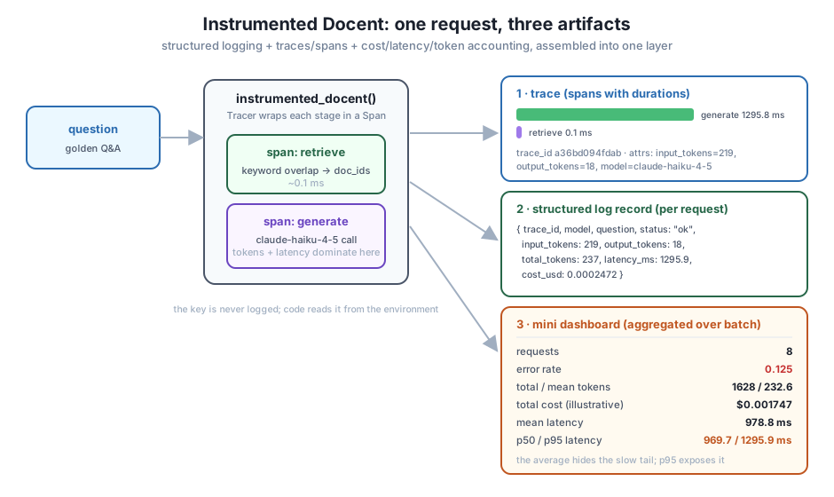
A dashboard you only glance at is decoration. The payoff of instrumentation is that it answers specific operational questions — the ones you’d ask at 2 a.m. when something is slow or expensive. We ask three, all answered directly from the frozen batch, no new model calls needed.

Which request was slowest, and where did the time go? We find the successful record with the highest latency and open its trace to see the span breakdown. Where do tokens and cost concentrate? We sort the successful records by cost and look at the top few. What would you optimize? The answer falls out of the first two.

ok_runs = [x for x in runs if x["record"]["status"] == "ok"]

# 1. slowest request -> open its trace
slow = max(ok_runs, key=lambda x: x["record"]["latency_ms"])
print(f"slowest: {slow['record']['latency_ms']}ms  trace {slow['record']['trace_id']}")
print(f"  q: {slow['record']['question']}")
for s in slow["trace"].spans:
    share = s.duration_ms / slow["record"]["latency_ms"]
    print(f"   span={s.name:9} {s.duration_ms:8.1f}ms  ({share:.0%} of request)")

# 2. where cost concentrates
top = sorted(ok_runs, key=lambda x: x["record"]["cost_usd"], reverse=True)[:3]
total = sum(x["record"]["cost_usd"] for x in ok_runs)
print("\ntop cost drivers:")
for x in top:
    r = x["record"]
    print(f"   ${r['cost_usd']:.6f}  {r['output_tokens']:>3} out-tok  {r['question'][:40]}")
print(f"top-3 share of spend: {sum(x['record']['cost_usd'] for x in top) / total:.0%}")

slowest: 1295.9ms  trace a36bd094fdab
  q: What HTTP status code does Meridian return when you exceed the rate limit?
   span=retrieve       0.1ms  (0% of request)
   span=generate    1295.8ms  (100% of request)

top cost drivers:
   $0.000334   42 out-tok  Can you change a database's region after
   $0.000269   22 out-tok  Which environment variable does the Pyth
   $0.000248   18 out-tok  How long are backups retained on the Sca

top-3 share of spend: 49%

This is the moment the whole module pays off: raw calls became an inspectable, costed, traced system, and now it answers questions. The slowest request’s trace is unambiguous — generate is 100% of the latency, retrieve is 0%. Whatever you do to make Docent faster, it will not be about retrieval; the lever is the model call (a smaller max_tokens, streaming so the user sees the first token sooner, or caching repeated prompts). The cost breakdown points the same way from a different angle: the three priciest requests account for about half of all spend, and they’re the ones with the most output tokens (the region question alone generated 42 output tokens versus 7–18 for the terse ones). Because output tokens are priced 5x input in our illustrative table, output length is the cost driver — the way to spend less is to prompt for shorter answers, not to shrink the docs you retrieve.

Two honesty notes. First, which request is slowest will change every run — latency is live, so on your machine the region or SDK question might top the list instead. That’s fine; the method is what’s stable — find the max, open its trace, read the span shares. Second, the cost and token numbers move a little run to run with answer length, but over any fixed collected batch the ranking and the aggregation are exact. The instrumentation didn’t make Docent better; it made Docent legible — and you can’t improve what you can’t see.

Practice Exercises#

Exercise 1: Add a token-budget attribute and flag over-budget requests#

Right now the layer records tokens but never judges them. Extend instrumented_docent so the generate span also records a boolean attribute over_budget, true when output_tokens exceeds a threshold you pick (say 30). Then, after the batch, print every request whose trace has an over-budget generate span. Confirm the region question — the longest answer in our run — is the one that trips it.

Exercise 2: Add p99 and explain why it needs more data#

The dashboard reports p50 and p95. Add a p99 latency line using the same pct helper. Then run the batch with only 7 successful requests and look at what p99 returns — you’ll find it equals the maximum. Explain why p99 is meaningless at this sample size, and estimate how many requests you’d need before p99 is a stable, trustworthy number.

Exercise 3: Group the dashboard by outcome status#

A single global dashboard blends successes and failures. Write a variant that computes the dashboard per status — one summary for ok requests, one for error — so you can see, for instance, that errors have zero cost and near-zero latency while successes carry all the tokens. Print both. Then argue why grouping (or “slicing”) a dashboard is often more useful than a single blended number.

Summary#

You built a real observability layer and wrapped it around Docent, combining everything Module 7 taught into one working system. You assembled the instrumentation layer — a Tracer and Span for timing, a structured log record for querying, and an illustrative cost helper for pricing — into instrumented_docent(question), which traces the retrieve and generate stages, logs one record per request, and returns (answer, trace, log_record) while never touching the API key. You ran it live on claude-haiku-4-5 over seven golden questions, collected every trace and record, and read one full trace and one full log record. You aggregated the batch into a mini dashboard — 8 requests, error rate 0.125 after injecting one failed call, 1628 total tokens, about $0.0017 total illustrative cost, mean latency 978.8 ms, p50 969.7 ms, p95 1295.9 ms — and confirmed it reproduces exactly (reproducible? True). And you used it: the slowest request’s trace showed generate was 100% of latency, and the top three requests drove roughly half of all spend, all on output tokens — telling you exactly where to optimize.

Key Concepts#

• Instrumentation layer — a thin wrapper of Tracer/Span, a structured log record, and a cost helper, assembled so every request emits a trace, a record, and (in aggregate) a dashboard; you build it once and every call inherits it.
• The three linked artifacts — trace, log record, and dashboard all share a trace_id; the trace shows where time went inside one request, the record is the queryable row, the dashboard is the batch summary.
• Collect-then-aggregate — freeze the live, varying batch once, then compute every metric deterministically over the frozen records so the dashboard reproduces (reproducible? True); keep the randomness in one clearly-labeled place.
• Percentiles over the mean — p50 and p95 expose the slow tail an average smooths away; percentiles need enough samples to be meaningful, which is why real dashboards aggregate over thousands of requests.
• A failure is a data point — catching errors into status: "error" records is what makes an error rate possible; deciding what a failed call contributes to each metric (counted for error rate, excluded from token/latency means) is a real observability judgment.

Why This Matters#

Everything before this module judged Docent against a dataset; this project makes Docent legible in production, which is a different and harder thing. A live LLM app that you can’t trace, log, or cost is a black box that works until it doesn’t, and when it slows down or runs up a bill you have nothing to look at. The layer you built turns every request into evidence — a trace that pinpoints where the time went, a record you can query, and a dashboard whose p95 and error rate you can alert on — and it does so cheaply, at the boundaries you control, without ever leaking a secret. That is the exact capability that separates a demo from a service: you can answer “which request was slow, where did the cost go, and what do I fix?” with data instead of a guess. Every production LLM system needs this instrumentation, and every optimization you make to one — smaller responses, streaming, caching, a cheaper model on easy queries — is a change you can only justify, and only verify, because you measured it first.

Continue Building Your Skills#

You just built the layer that turns a working LLM app into an operable one. It wraps Docent’s retrieve and generate stages in timed spans, emits a structured record for every request, prices each call, and rolls a batch up into a dashboard with the percentiles and error rate an on-call engineer actually watches — and it does all of it without ever reading or logging the API key. You proved the aggregation reproduces exactly over a frozen batch, then used it to find that the model call is 100% of Docent’s latency and output length is its main cost driver: two optimization decisions you could only make because you measured them. Carry the instinct forward — when you ship an LLM feature, instrument it before you tune it, because the trace, the cost, and the p95 are what tell you whether your change helped or just felt faster. In Module 8, this instrumentation stops being something you inspect after the fact and becomes something that watches in real time: monitoring that alerts on these metrics and guardrails that act on them before a bad response reaches a user.