Lesson 4 - The Airflow UI Tour

Welcome to the Airflow UI Tour#

Lesson 3 proved cityflow_hello ran and succeeded, entirely through the CLI. Everything that lesson confirmed with airflow dags list-runs and airflow tasks states-for-dag-run is also sitting in the same webserver UI Lesson 2 first logged into — this lesson is a tour of exactly where, with real screenshots of the real, finished run.

By the end of this lesson, you will be able to:

• Read a DAG’s row in the DAGs list — run counts, last run time, recent task dots
• Read a DAG run’s Grid view and tell, at a glance, which tasks succeeded, failed, or never ran
• Find and read a specific task’s real log output from inside the UI

The DAGs List, No Longer Empty#

Lesson 2 ended on a DAGs list with zero rows. After Lesson 3, the same page looks like this:

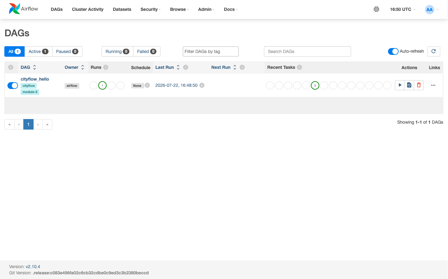
Read the row left to right: the toggle on the left is the pause switch Lesson 3 flipped with airflow dags unpause. cityflow and module-2 are the tags set in the @dag(...) decorator. Runs shows one green circle — Lesson 3’s single successful run — with two empty outlines beside it reserved for whatever runs come next. Schedule reads None, matching schedule=None in the DAG’s code: this DAG only ever runs when triggered, on purpose. Recent Tasks shows three small circles, all green — one per task, confirming what airflow tasks states-for-dag-run already told you in text.

The Grid View: One Run, Every Task#

Click the DAG’s name and Airflow’s default view is the Grid — a run-by-run, task-by-task history:

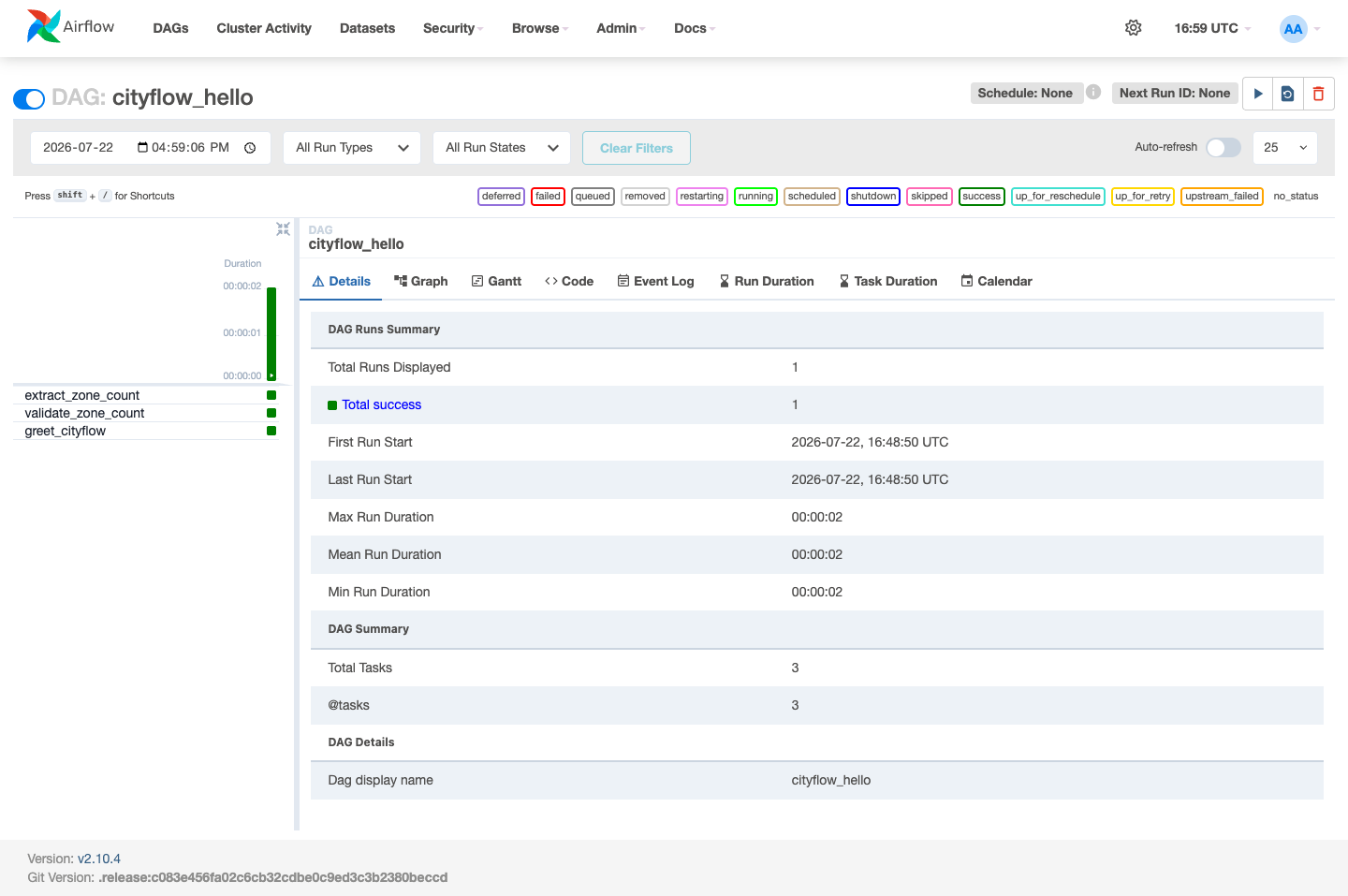
Each row on the left is one task; each column would be one run (there’s only one so far). The color is the same vocabulary Airflow uses everywhere — the legend above the grid (success, failed, running, queued, and so on) is the same set of states airflow tasks states-for-dag-run printed as plain text in Lesson 3. The Details panel confirms the same facts in numbers: Total Runs Displayed: 1, Total success: 1, Total Tasks: 3, Max/Mean/Min Run Duration: 00:00:02 — this DAG really did finish in about two seconds, matching the millisecond timestamps Lesson 3’s CLI output showed.

Reading a Real Task’s Log#

Click any green square and a task detail panel opens with a Logs tab — the same log file Lesson 3 already read through docker exec ... cat, now in the browser:

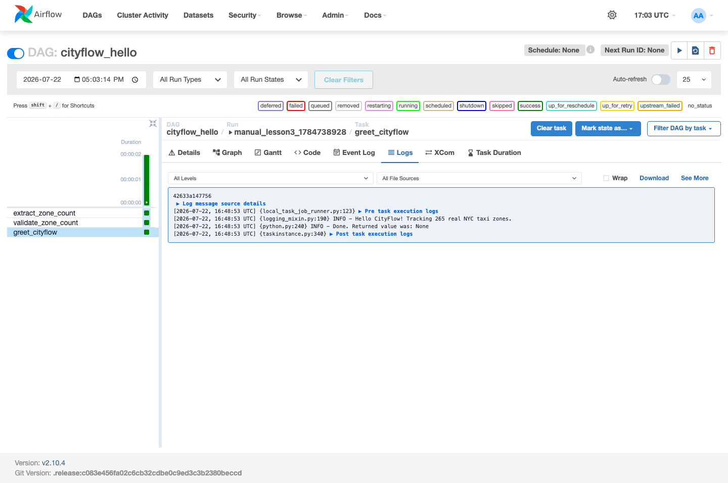
This is not a mockup of what a log page could look like — it’s the literal file Airflow’s task process wrote to disk, rendered by the webserver. The line Hello CityFlow! Tracking 265 real NYC taxi zones. is the exact print() statement from greet_cityflow, at the exact timestamp it ran. Everything above it (Pre task execution logs) and below it (Done. Returned value was: None, Post task execution logs) is Airflow’s own instrumentation — proof of when the task actually started, what it returned, and when it actually finished, all without you having to add a single line of logging code yourself.

Key Takeaways#

• The DAGs list’s Runs and Recent Tasks columns are a compact summary — green means success, and the count next to All/Active/Paused at the top is a real, live count, not a static label.
• The Grid view is a task-by-task, run-by-run history; its Details panel restates the same facts the CLI already gave you (run count, success count, task count, durations) in a different form — useful for confirming the UI and CLI genuinely agree.
• A task’s Logs tab shows the actual file Airflow’s task process wrote — the same content docker exec ... cat <logfile> would show, just rendered in the browser with Airflow’s own pre/post-execution markers around it.
• Nothing in this lesson’s screenshots is staged — every one is Lesson 3’s real, already-finished cityflow_hello run, captured live from the running webserver.

Exercises#

Exercise 1 — In the real UI, open cityflow_hello’s Grid view and click the Code tab. Confirm the source shown there is character-for-character the same cityflow_hello_dag.py this lesson describes — the webserver reads DAG source directly from the mounted dags/ folder, the same one the scheduler parses.

Exercise 2 — Open the Details tab (not Logs) for the extract_zone_count task specifically, and find its Duration. Compare it to validate_zone_count’s duration — which task took longer, and does that match what you’d expect given extract_zone_count reads a file from disk while validate_zone_count only does an in-memory comparison?

Exercise 3 — In the Logs tab for any task, click Download. Open the downloaded file in a text editor and confirm it’s identical to what the browser rendered — proof the UI isn’t summarizing or reformatting the log, just displaying the real file.