Title here
Summary here
Module 2 Lesson 4 already covered the Grid view’s basics — task rows, colored squares, the Details panel. What it didn’t cover is the pair of views built specifically for timing: the Grid page’s Task Duration chart, which plots exactly how long each task took, and its Gantt view, which lays every task out on a real timeline. Both need something Modules 2-5’s small DAGs never had much of: tasks whose real durations are genuinely different from each other.
By the end of this lesson, you will be able to:
cityflow_monitoring_demo_dag.py is the same real ingest → validate → transform → load shape Module 5 built, run here against CityFlow’s entire real January 2024 month instead of a few days — specifically so the four tasks land at genuinely different durations: a large parquet read and a five-check pass over millions of real rows, next to a small groupby and a small Postgres insert.
# gate: skip
"""CityFlow's real monitoring demo (Module 6 Lesson 3).

The same real ingest -> validate -> transform -> load shape Module 5 built,
run here over CityFlow's full real January 2024 taxi month (not a single
day) specifically so the four tasks land at genuinely different real
durations -- a large parquet read and a five-check pass over ~2.96 million
real rows next to a small groupby and a small Postgres insert. The point of
this DAG isn't new pipeline logic, it's giving the Grid and Gantt views in
this lesson a real duration spread worth looking at."""
from datetime import datetime

from airflow.decorators import dag, task

PARQUET_PATH = "/opt/airflow/dags/data/yellow_tripdata_2024-01.parquet"
ZONE_LOOKUP_PATH = "/opt/airflow/dags/data/taxi_zone_lookup.csv"
WORK_DIR = "/opt/airflow/dags/data/work/monitoring_demo"
CLEAN_TRIPS_PATH = f"{WORK_DIR}/clean_trips.csv"
TRANSFORMED_PATH = f"{WORK_DIR}/daily_borough_summary.csv"
KEEP_COLUMNS = [
    "tpep_pickup_datetime", "tpep_dropoff_datetime", "passenger_count",
    "trip_distance", "PULocationID", "DOLocationID", "fare_amount", "total_amount",
]
POSTGRES_CONN_ID = "cityflow_postgres"
TABLE_NAME = "cityflow_monitoring_demo_summary"


@dag(
    dag_id="cityflow_monitoring_demo",
    schedule=None,
    start_date=datetime(2026, 1, 1),
    catchup=False,
    tags=["cityflow", "module-6", "monitoring"],
)
def cityflow_monitoring_demo_dag():
    @task
    def ingest_full_month() -> int:
        import os

        import pandas as pd

        raw = pd.read_parquet(PARQUET_PATH, columns=KEEP_COLUMNS)
        os.makedirs(WORK_DIR, exist_ok=True)
        raw.to_csv(f"{WORK_DIR}/raw_trips.csv", index=False)
        print(f"ingest_full_month: read {len(raw)} real CityFlow trips for the whole real January 2024 month")
        return len(raw)

    @task
    def validate_full_month(ingested_rows: int) -> dict:
        import sys

        import pandas as pd

        sys.path.insert(0, "/opt/airflow/dags")
        import cityflow_validation_logic as vlogic

        trips = pd.read_csv(f"{WORK_DIR}/raw_trips.csv", parse_dates=["tpep_pickup_datetime", "tpep_dropoff_datetime"])
        assert len(trips) == ingested_rows
        report, any_fail = vlogic.validate_trips_df(trips)
        trips[~any_fail].to_csv(CLEAN_TRIPS_PATH, index=False)
        print(f"validate_full_month: {report}")
        return report

    @task
    def transform_full_month(validation_report: dict) -> dict:
        import pandas as pd

        clean = pd.read_csv(CLEAN_TRIPS_PATH, parse_dates=["tpep_pickup_datetime", "tpep_dropoff_datetime"])
        assert len(clean) == validation_report["rows_passed"]

        zones = pd.read_csv(ZONE_LOOKUP_PATH)[["LocationID", "Borough"]].rename(columns={"LocationID": "PULocationID"})
        clean = clean.merge(zones, on="PULocationID", how="left")
        clean["Borough"] = clean["Borough"].fillna("Unknown")
        clean["pickup_date"] = clean["tpep_pickup_datetime"].dt.date

        agg = clean.groupby(["pickup_date", "Borough"]).agg(
            trip_count=("fare_amount", "size"),
            avg_fare_amount=("fare_amount", "mean"),
            total_revenue=("total_amount", "sum"),
        ).reset_index()
        for col in ("avg_fare_amount", "total_revenue"):
            agg[col] = agg[col].round(2)
        agg.to_csv(TRANSFORMED_PATH, index=False)
        total_trip_count = int(agg["trip_count"].sum())
        assert total_trip_count == validation_report["rows_passed"]
        print(f"transform_full_month: {len(agg)} day/borough rows, total_trip_count={total_trip_count}")
        return {"summary_rows": len(agg), "total_trip_count": total_trip_count}

    @task
    def load_full_month(transform_result: dict) -> int:
        import pandas as pd
        from airflow.providers.postgres.hooks.postgres import PostgresHook

        summary = pd.read_csv(TRANSFORMED_PATH)
        hook = PostgresHook(postgres_conn_id=POSTGRES_CONN_ID)
        hook.run(f"DROP TABLE IF EXISTS {TABLE_NAME};")
        hook.run(f"""
            CREATE TABLE {TABLE_NAME} (
                id SERIAL PRIMARY KEY, pickup_date DATE NOT NULL, borough TEXT NOT NULL,
                trip_count INTEGER NOT NULL, avg_fare_amount REAL, total_revenue REAL
            );
        """)
        rows = list(summary[["pickup_date", "Borough", "trip_count", "avg_fare_amount", "total_revenue"]].itertuples(index=False, name=None))
        hook.insert_rows(table=TABLE_NAME, rows=rows,
                          target_fields=["pickup_date", "borough", "trip_count", "avg_fare_amount", "total_revenue"],
                          commit_every=50)
        row_count = hook.get_first(f"SELECT COUNT(*) FROM {TABLE_NAME};")[0]
        assert row_count == len(summary)
        print(f"load_full_month: loaded {row_count} real day/borough rows into {TABLE_NAME}")
        return row_count

    load_full_month(transform_full_month(validate_full_month(ingest_full_month())))


cityflow_monitoring_demo_dag()
Note the validate_full_month task: it imports cityflow_validation_logic (Lesson 1) rather than reimplementing the five checks — one real function, already unit-tested, used everywhere it’s needed.
# gate: setup: docker rm -f cityflow-lessons-db >/dev/null 2>&1; docker run -d --name cityflow-lessons-db -e POSTGRES_USER=cityflow -e POSTGRES_PASSWORD=cityflow -e POSTGRES_DB=cityflow -p 55432:5432 postgres:13 >/dev/null && sleep 4
# gate: teardown: docker rm -f cityflow-lessons-db >/dev/null 2>&1
import json
import subprocess
import time

dag_id = "cityflow_monitoring_demo"

subprocess.run(["docker", "exec", "airflow-local-airflow-scheduler-1", "airflow", "dags", "unpause", dag_id],
                capture_output=True, text=True, check=True)

run_id = f"lesson3_m6_verify_{int(time.time())}"
trigger = subprocess.run(
    ["docker", "exec", "airflow-local-airflow-scheduler-1", "airflow", "dags", "trigger", dag_id, "--run-id", run_id],
    capture_output=True, text=True,
)
if trigger.returncode != 0:
    subprocess.run(["docker", "exec", "airflow-local-airflow-scheduler-1", "airflow", "dags", "reserialize"],
                    capture_output=True, text=True, check=True)
    subprocess.run(
        ["docker", "exec", "airflow-local-airflow-scheduler-1", "airflow", "dags", "trigger", dag_id, "--run-id", run_id],
        capture_output=True, text=True, check=True,
    )
print(f"triggered {dag_id!r} as {run_id!r}")

deadline = time.time() + 300
state = "queued"
while state not in ("success", "failed") and time.time() < deadline:
    time.sleep(3)
    r = subprocess.run(
        ["docker", "exec", "airflow-local-airflow-scheduler-1", "airflow", "dags", "list-runs", "-d", dag_id, "--output", "json"],
        capture_output=True, text=True, check=True,
    )
    runs = json.loads(r.stdout)
    match = [x for x in runs if x["run_id"] == run_id]
    state = match[0]["state"] if match else "queued"
print(f"run {run_id!r} reached state: {state}")
assert state == "success", f"expected success, got {state}"

r = subprocess.run(
    ["docker", "exec", "airflow-local-airflow-scheduler-1", "airflow", "tasks", "states-for-dag-run", dag_id, run_id],
    capture_output=True, text=True, check=True,
)
print(r.stdout)
triggered 'cityflow_monitoring_demo' as 'lesson3_m6_verify_1784925837'
run 'lesson3_m6_verify_1784925837' reached state: success
dag_id | execution_date | task_id | state | start_date | end_date
=========================+===========================+======================+=========+==================================+=================================
cityflow_monitoring_demo | 2026-07-24T20:43:58+00:00 | validate_full_month | success | 2026-07-24T20:44:10.620827+00:00 | 2026-07-24T20:44:22.843157+00:00
cityflow_monitoring_demo | 2026-07-24T20:43:58+00:00 | ingest_full_month | success | 2026-07-24T20:43:59.726137+00:00 | 2026-07-24T20:44:09.992127+00:00
cityflow_monitoring_demo | 2026-07-24T20:43:58+00:00 | transform_full_month | success | 2026-07-24T20:44:23.911888+00:00 | 2026-07-24T20:44:27.692736+00:00
cityflow_monitoring_demo | 2026-07-24T20:43:58+00:00 | load_full_month | success | 2026-07-24T20:44:27.788473+00:00 | 2026-07-24T20:44:28.188364+00:00Doing the subtraction by hand from these real timestamps: ingest_full_month ≈ 10.27s, validate_full_month ≈ 12.22s, transform_full_month ≈ 3.78s, load_full_month ≈ 0.40s — a real, roughly 30x spread between the slowest and fastest task, entirely from real work at real scale (2,964,624 rows ingested and checked five different ways).
The Grid page has a dedicated tab for exactly this comparison — not the colored squares themselves (those encode state: green, red, orange), but a separate Task Duration view plotting each task’s real duration as its own point:
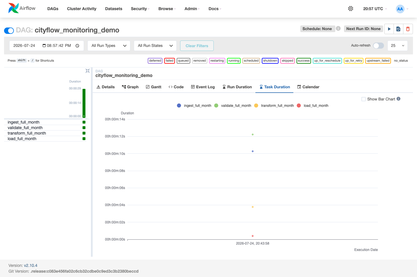
This view exists because the Grid’s own squares can’t show duration directly — a green square means “succeeded,” whether that took 400 milliseconds or 12 seconds. Task Duration answers the question the squares can’t: which task is actually the bottleneck? Here it’s unambiguous — validate_full_month (checking 2,964,624 rows five different ways) and ingest_full_month (reading the whole real parquet file) dominate; transform_full_month’s groupby and load_full_month’s small Postgres insert barely register by comparison.
The Gantt view answers a different question: not “how long did each task take” but “when, exactly, did each one run relative to the others”:
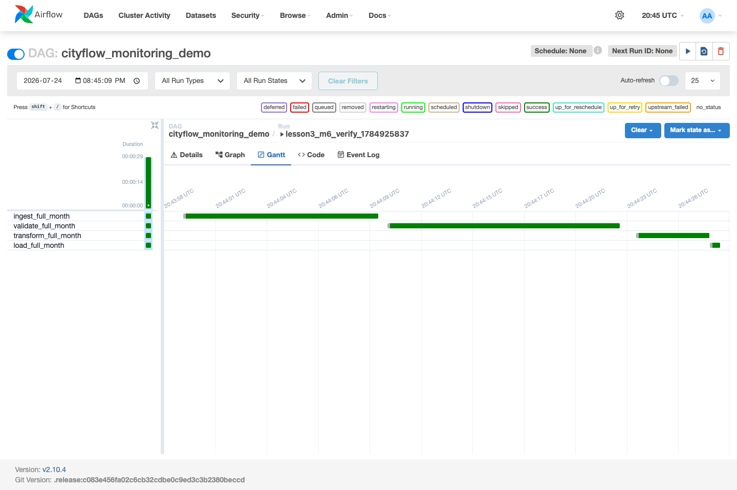
This is where the difference from Grid actually shows up. Grid’s squares tell you each task succeeded; Gantt tells you when, in real wall-clock time, against every other task’s real timing — and for a linear DAG like this one (ingest → validate → transform → load, each depending on the one before it), that means you can see the real, small gaps between one task ending and the next beginning: ingest_full_month ends around 20:44:09.99, validate_full_month doesn’t start until 20:44:10.62 — about 630ms of real scheduler overhead between “the upstream task finished” and “the next task actually started,” invisible in Grid’s squares but plainly visible as a gap in Gantt’s timeline. For a DAG with tasks that run in parallel (Module 3’s branching DAG, for instance), that same Gantt view would show two bars overlapping in time instead of a gap between them — the one shape Grid’s per-run squares can never show at all, since a square only ever represents one task’s overall state, not its position on a shared timeline.
ingest_full_month and validate_full_month); for a DAG with parallel branches, it would instead reveal real overlap — neither is visible in Grid’s per-task squares.Exercise 1 — Open the real Gantt view for this run yourself and hover over the validate_full_month bar. Confirm the tooltip’s start/end times match the CLI table’s start_date/end_date for that task exactly.
Exercise 2 — Re-trigger cityflow_monitoring_demo a second time and compare its real durations to the ones recorded in this lesson. Are they close? What’s a plausible reason two runs of the exact same code over the exact same file might still differ by a second or two (hint: what else was this machine doing during each run)?
Exercise 3 — Look at Module 3 Lesson 3’s branching-graph-view.png (cityflow_branching_demo, which really does run two tasks in parallel) and imagine its Gantt view. Based on this lesson’s explanation, would you expect to see two bars with a gap between them, or two bars overlapping? Open that DAG’s real Gantt view in the UI (.airflow-local/dags/cityflow_branching_dag.py is still live) to check your prediction.
Keep DATATWEETS free. Help fund practical data, AI, and engineering lessons for learners worldwide.
