Lesson 2 - How Polars Differs from Python and Pandas

Welcome to How Polars Differs from Python and Pandas#

Lesson 1 named two problems: loops get slow, and pandas’s index model creates silent bugs. This lesson measures the first one honestly, with a stopwatch, and explains the second one properly: what does it actually mean that Polars has no index?

By the end of this lesson, you will be able to:

• Run the same real aggregation task as a plain Python loop and as Polars, and read an honest, measured timing result
• Explain why the difference isn’t really about Python being “slow” — it’s about where the work happens
• Describe what “no index” means for a Polars DataFrame and why that removes a whole category of pandas bug
• Recognize when a loop is fine and when reaching for Polars actually matters

Let’s begin with a task sized the way Thistlewood Goods’ real order data will be by the time you finish this module: not four rows, but a million.

The Task: Revenue by Category, at Real Scale#

Thistlewood Goods logs every item sold as an order line — one row per product per order, with a category and a dollar amount. Add up revenue and line count per category, across a file with a million such rows. This is about as basic as data tasks get, and it’s exactly the kind of thing that feels instant on a spreadsheet of 50 rows and very much not instant at a million.

Setting Up the Comparison#

First, generate a realistic-sized file to work with — a million order lines, spread across Thistlewood’s eight categories, written to a real CSV on disk:

import csv
import os
import random
import tempfile

random.seed(42)
CATEGORIES = ["Kitchen", "Bath", "Bedding", "Lighting", "Storage", "Decor", "Furniture", "Outdoor"]
N_LINES = 1_000_000

WORKDIR = os.path.join(tempfile.gettempdir(), "thistlewood_bench")
os.makedirs(WORKDIR, exist_ok=True)
PATH = os.path.join(WORKDIR, "order_lines_bench.csv")

with open(PATH, "w", newline="") as f:
    writer = csv.writer(f)
    writer.writerow(["category", "amount"])
    for _ in range(N_LINES):
        writer.writerow([random.choice(CATEGORIES), round(random.uniform(8, 450), 2)])

print(f"wrote {N_LINES:,} order-line rows to {PATH}")

wrote 1,000,000 order-line rows to /tmp/thistlewood_bench/order_lines_bench.csv

That’s a real file on disk, a little over 20 MB, with a million real rows in it. Both approaches below read this exact same file.

Plain Python: Read and Loop#

The straightforward way to answer “revenue and line count per category” without any library beyond the standard one: open the file, read it row by row, and keep a running total in a couple of dictionaries.

import csv
import os
import tempfile
import time

WORKDIR = os.path.join(tempfile.gettempdir(), "thistlewood_bench")
PATH = os.path.join(WORKDIR, "order_lines_bench.csv")

start = time.perf_counter()
totals = {}
counts = {}
with open(PATH, newline="") as f:
    reader = csv.reader(f)
    next(reader)  # header
    for category, amount in reader:
        amount = float(amount)
        totals[category] = totals.get(category, 0.0) + amount
        counts[category] = counts.get(category, 0) + 1
loop_seconds = time.perf_counter() - start

print(f"plain Python loop: {loop_seconds:.3f} seconds")
for category in sorted(totals):
    print(f"  {category:10s} revenue=${totals[category]:>13,.2f}  lines={counts[category]:,}")

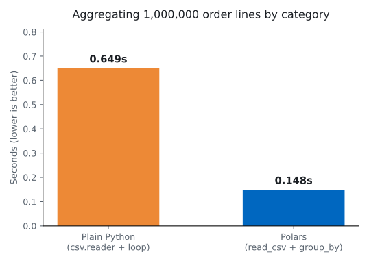
plain Python loop: 0.649 seconds
  Bath       revenue=$28,652,173.11  lines=125,138
  Bedding    revenue=$28,567,358.34  lines=124,721
  Decor      revenue=$28,711,888.30  lines=125,431
  Furniture  revenue=$28,566,041.09  lines=125,051
  Kitchen    revenue=$28,613,514.84  lines=125,189
  Lighting   revenue=$28,513,400.32  lines=124,557
  Outdoor    revenue=$28,448,949.05  lines=124,429
  Storage    revenue=$28,742,899.55  lines=125,484

Nothing wrong with this code. It’s clear, it’s correct, and it produces the right answer. It just spends 0.649 seconds doing it — on this run, on this machine, for one million rows. Every one of those million iterations re-enters the Python interpreter, converts a string to a float, does two dictionary lookups and two dictionary writes. None of that work is expensive on its own; there’s just a lot of it, one row at a time.

Polars: Read and Group#

Here’s the same question, answered with Polars:

import os
import tempfile
import time

import polars as pl

WORKDIR = os.path.join(tempfile.gettempdir(), "thistlewood_bench")
PATH = os.path.join(WORKDIR, "order_lines_bench.csv")

start = time.perf_counter()
lines = pl.read_csv(PATH)
by_category = (
    lines.group_by("category")
    .agg(pl.col("amount").sum().round(2).alias("revenue"), pl.len().alias("lines"))
    .sort("category")
)
polars_seconds = time.perf_counter() - start

print(f"Polars (read_csv + group_by): {polars_seconds:.3f} seconds")
print(by_category)

Polars (read_csv + group_by): 0.148 seconds
shape: (8, 3)
┌───────────┬──────────┬────────┐
│ category  ┆ revenue  ┆ lines  │
│ ---       ┆ ---      ┆ ---    │
│ str       ┆ f64      ┆ u32    │
╞═══════════╪══════════╪════════╡
│ Bath      ┆ 2.8652e7 ┆ 125138 │
│ Bedding   ┆ 2.8567e7 ┆ 124721 │
│ Decor     ┆ 2.8712e7 ┆ 125431 │
│ Furniture ┆ 2.8566e7 ┆ 125051 │
│ Kitchen   ┆ 2.8614e7 ┆ 125189 │
│ Lighting  ┆ 2.8513e7 ┆ 124557 │
│ Outdoor   ┆ 2.8449e7 ┆ 124429 │
│ Storage   ┆ 2.8743e7 ┆ 125484 │
└───────────┴──────────┴────────┘

Same file, same eight categories, same totals — Bath’s revenue is $28,652,173.11 in both results, down to the cent. What’s different is that it took 0.148 seconds instead of 0.649: 4.4 times faster, measured on this run, on this exact file.

Why the Gap: Where the Work Actually Happens#

It’s tempting to say “Polars is written in Rust, Rust is fast, that’s the whole story” — and compiled code is part of it, but it’s not the interesting part. You could write the loop above in a faster language and still lose to Polars at scale, because the real difference is architectural, not just a language choice.

One Interpreter Trip vs. Many#

The plain Python loop above does exactly one thing about a million times: run a small chunk of Python bytecode. Each float(amount), each dictionary .get(...), each assignment — the Python interpreter has to dispatch every one of those individually, checking types and managing memory as it goes. That dispatch cost doesn’t care whether the actual arithmetic is trivial; it’s paid per operation, every time.

Polars’s group_by(...).agg(...) call is a single instruction from Python’s point of view. Python calls into Polars once, and everything after that — reading the CSV, parsing a million strings into numbers, splitting rows into eight groups, summing within each group — happens inside compiled code that never has to ask the Python interpreter what to do next. The million-row loop is still there; it’s just not a Python loop anymore.

No Index, No Ambiguity#

This section is about correctness, not the speed you just measured — worth keeping separate, since they come from different parts of Polars’s design. Lesson 1 showed a pandas bug rooted in chained assignment and copy/view ambiguity: products[condition] can return a view or a copy depending on internals you can’t easily predict, and assigning into the result of that first indexing step never reliably writes back to products. Pandas’s row-label index is a related but separate piece of machinery — it exists to align two Series by label during arithmetic, a genuinely useful feature — and it introduces its own class of surprise (two Series with mismatched labels silently producing NaNs on alignment), but it isn’t itself the direct cause of the copy/view trap.

Polars sidesteps both. A Polars DataFrame’s rows are identified purely by their position — row 0, row 1, row 2 — the same way a plain Python list is, so there’s no label space to align or reconcile. And because every Polars transformation takes a DataFrame in and returns a complete new DataFrame out, there’s no partial, aliased view that might or might not still be connected to where it came from — the chained-assignment trap from Lesson 1 has nothing to attach to. Two separate simplifications, both removing a real category of surprise.

When a Loop Is Genuinely Fine#

None of this means loops are wrong. If you’re processing 20 rows once, in a one-off script, a plain Python loop is completely reasonable — it’s readable, and 20 iterations of interpreter overhead is nothing. The lesson from this benchmark isn’t “never loop”; it’s “know where the cost actually comes from, so you can tell when it’s about to matter.” Thistlewood Goods’ real order history, which you’ll build in Lesson 5, is already at a scale where the difference is worth having in your toolkit.

Practice Exercises#

Exercise 1: Re-run and compare#

Run both scripts above yourself, back to back, on your own machine. Report your own measured times and the speedup ratio. Are they close to 4.4x, or different? Note anything about your machine (SSD vs. spinning disk, how many CPU cores) that might explain a difference from this lesson’s numbers.

Exercise 2: Scale it down and up#

Change N_LINES to 10_000 and re-run both versions. Then try 5_000_000. What happens to the gap between the two approaches as the row count shrinks and grows? Write one sentence explaining why the gap doesn’t stay constant.

Summary#

A plain Python loop and Polars can produce the exact same correct answer — this lesson’s benchmark proved that down to the cent — but they get there through very different amounts of interpreter overhead. Measured on one million order lines, a csv.reader loop took 0.649 seconds; Polars’s read_csv plus group_by took 0.148 seconds, about 4.4 times faster on that run. The deeper reason isn’t just “compiled code is fast” — it’s that Python is called once instead of a million times, with the per-row work happening in compiled code the whole way through. Separately, and for a different reason, Polars’s no-index model is why the chained-assignment bug from Lesson 1 can’t happen here in the first place — that’s a correctness win, not the source of this speed measurement.

Key Concepts#

• Interpreter overhead — the fixed cost of dispatching a Python bytecode operation, paid once per loop iteration regardless of how trivial the operation is.
• No-index model — Polars identifies rows purely by position, with no separate label space to align or reconcile, unlike pandas’s index.
• Vectorized / single-call execution — Polars’s group_by(...).agg(...) crosses from Python into compiled code exactly once, doing the per-row work internally instead of via a Python-level loop.

Why This Matters#

Knowing why Polars is fast, not just that it’s fast, tells you when the speedup actually applies. A tool that’s fast for mysterious reasons gets used superstitiously; a tool whose speed you understand gets used well — reached for when the row count justifies it, skipped without guilt when it doesn’t.

Continue Building Your Skills#

You’ve seen the “why.” Lesson 3 gets your hands on the keyboard: a real local project, a virtual environment, and a folder structure ready for the Thistlewood Goods pipeline you’ll build for the rest of this module.