Lesson 4 - Install Polars and Run Your First Pipeline

Welcome to Install Polars and Run Your First Pipeline#

The project folder from Lesson 3 is ready. This lesson puts Polars into it for real, confirms the install actually worked, and then builds the smallest genuine pipeline there is: read some data, keep only the rows you care about, summarize what’s left, and print the answer. Every step here is real code you run yourself, not a description of what it would do.

By the end of this lesson, you will be able to:

• Install Polars into your project’s virtual environment with pip
• Verify the installed version for real, from the command line and from Python
• Write a four-stage pipeline — read, filter, aggregate, print — using Polars expressions
• Recognize this exact read/filter/aggregate/print shape, because you’ll use it in every remaining lesson of this course

Make sure your virtual environment from Lesson 3 is activated before you start — you should see its path when you run which python.

Installing Polars#

With .venv activated, installing Polars is one command:

pip install polars

pip resolves and downloads the package, and within a few seconds you have a working Polars install — there’s no compiler to configure and no separate native library to install alongside it; the package ships everything it needs.

Recording the Dependency#

Now that something is actually installed, capture it in requirements.txt the way Lesson 3 set up:

pip freeze > requirements.txt
cat requirements.txt

polars==1.43.0
polars-runtime-32==1.43.0

polars-runtime-32 is Polars’s own compiled runtime, installed automatically alongside the polars package itself — pip freeze lists it separately because it’s technically its own distribution, even though you never import it directly. (Your exact versions may be newer, depending on when you’re reading this — that’s fine. What matters is that the file now records precisely what your environment has, so anyone else who runs pip install -r requirements.txt gets the same thing.)

Verifying the Install for Real#

Don’t take pip’s word for it — check from inside Python that the import actually works and see exactly which version landed:

import polars
print(polars.__version__)

1.43.0

If this line raises ModuleNotFoundError instead, the most common cause is an unactivated virtual environment — double check which python points inside .venv/ before re-running pip install polars.

What Actually Got Installed#

pip show reveals what a package pulled in alongside itself:

pip show polars

Name: polars
Version: 1.43.0
Summary: Blazingly fast DataFrame library
Home-page: https://www.pola.rs/
Requires: polars-runtime-32
Required-by:

One real dependency, polars-runtime-32 (Polars’s own compiled runtime component) — that’s the entire chain. Compare that to pandas, whose own pip show pandas lists Requires: numpy, python-dateutil (and those two bring in further dependencies of their own). Fewer dependencies mostly means less that can go wrong during install — less version-resolution work for pip to do, and fewer packages that could each independently break on a given platform. It’s a small, concrete piece of evidence for the same design philosophy Lesson 1 introduced — Polars is built as a complete, self-contained tool, not a layer added on top of an existing stack — though installed dependency count on its own doesn’t tell you how much of that code actually runs in a given program.

Your First Real Pipeline#

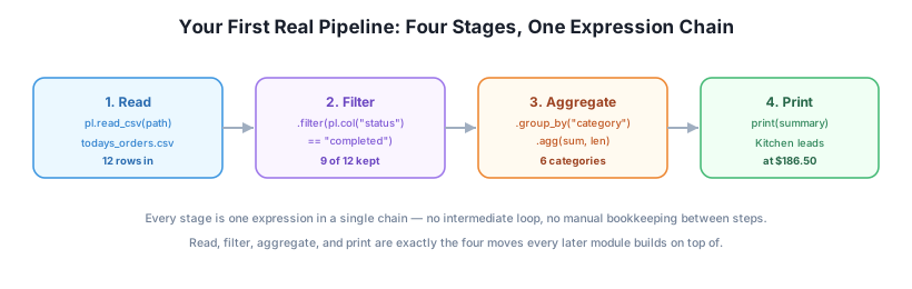
Time to use it. The shape below — read, filter, aggregate, print — is the single most common pattern in data work, and you’ll see it again in almost every lesson from here on, growing more sophisticated each time. This version keeps it as small as it can honestly be.

The Scenario#

Imagine it’s the end of a morning at Thistlewood Goods, and you have a small CSV of that morning’s orders: which category, which channel, what status, and how much. You want to know real revenue by category — but “real revenue” has to exclude orders that were cancelled or are still pending, since those haven’t actually happened yet.

import os
import tempfile

import polars as pl

WORKDIR = os.path.join(tempfile.gettempdir(), "thistlewood_first_pipeline")
os.makedirs(WORKDIR, exist_ok=True)
PATH = os.path.join(WORKDIR, "todays_orders.csv")

# A small, hand-written sample of one morning's Thistlewood Goods orders.
csv_text = """order_id,category,channel,status,amount
O1001,Kitchen,web,completed,64.00
O1002,Bath,store,completed,38.00
O1003,Kitchen,web,cancelled,72.00
O1004,Outdoor,phone,completed,26.00
O1005,Lighting,web,completed,145.00
O1006,Kitchen,store,completed,58.50
O1007,Bath,web,pending,42.00
O1008,Decor,web,completed,89.00
O1009,Kitchen,phone,completed,64.00
O1010,Outdoor,store,completed,112.00
O1011,Lighting,web,cancelled,145.00
O1012,Bedding,web,completed,97.50
"""
with open(PATH, "w") as f:
    f.write(csv_text)

Nothing about that setup is Polars yet — it’s just writing a small real CSV to disk so the next part has something genuine to read. In a real project this file would already exist; here, writing it explicitly means you can run this lesson exactly as shown and get exactly this lesson’s numbers.

Stage 1: Read#

orders = pl.read_csv(PATH)
print(f"read {orders.height} rows from {PATH}")
print(orders)

read 12 rows from /tmp/thistlewood_first_pipeline/todays_orders.csv
shape: (12, 5)
┌──────────┬──────────┬─────────┬───────────┬────────┐
│ order_id ┆ category ┆ channel ┆ status    ┆ amount │
│ ---      ┆ ---      ┆ ---     ┆ ---       ┆ ---    │
│ str      ┆ str      ┆ str     ┆ str       ┆ f64    │
╞══════════╪══════════╪═════════╪═══════════╪════════╡
│ O1001    ┆ Kitchen  ┆ web     ┆ completed ┆ 64.0   │
│ O1002    ┆ Bath     ┆ store   ┆ completed ┆ 38.0   │
│ O1003    ┆ Kitchen  ┆ web     ┆ cancelled ┆ 72.0   │
│ O1004    ┆ Outdoor  ┆ phone   ┆ completed ┆ 26.0   │
│ O1005    ┆ Lighting ┆ web     ┆ completed ┆ 145.0  │
│ …        ┆ …        ┆ …       ┆ …         ┆ …      │
│ O1008    ┆ Decor    ┆ web     ┆ completed ┆ 89.0   │
│ O1009    ┆ Kitchen  ┆ phone   ┆ completed ┆ 64.0   │
│ O1010    ┆ Outdoor  ┆ store   ┆ completed ┆ 112.0  │
│ O1011    ┆ Lighting ┆ web     ┆ cancelled ┆ 145.0  │
│ O1012    ┆ Bedding  ┆ web     ┆ completed ┆ 97.5   │
└──────────┴──────────┴─────────┴───────────┴────────┘

One function call, pl.read_csv, and Polars has inferred the schema — notice str for the text columns and f64 for amount — without you specifying a single type. The … row in the middle is Polars itself abbreviating a DataFrame that’s taller than its default print height; the data underneath is still all 12 rows, as orders.height confirms.

Stage 2: Filter#

Two of the twelve orders are cancelled, one is pending — none of those three represent real revenue yet:

completed = orders.filter(pl.col("status") == "completed")
print(f"{completed.height} of {orders.height} orders were completed")

9 of 12 orders were completed

pl.col("status") == "completed" builds a boolean expression, and .filter(...) keeps only the rows where it’s true — no manual index bookkeeping, no separate boolean array to keep track of.

Stage 3: Aggregate#

Now group what’s left by category and total it up:

summary = (
    completed.group_by("category")
    .agg(pl.col("amount").sum().alias("revenue"), pl.len().alias("orders"))
    .sort("revenue", descending=True)
)

group_by("category") buckets rows by category, and .agg(...) computes, for each bucket, the summed amount (aliased to revenue) and a row count (pl.len(), aliased to orders) — both from the same .agg(...) call.

Stage 4: Print#

print("Revenue by category (completed orders only):")
print(summary)

Revenue by category (completed orders only):
shape: (6, 3)
┌──────────┬─────────┬────────┐
│ category ┆ revenue ┆ orders │
│ ---      ┆ ---     ┆ ---    │
│ str      ┆ f64     ┆ u32    │
╞══════════╪═════════╪════════╡
│ Kitchen  ┆ 186.5   ┆ 3      │
│ Lighting ┆ 145.0   ┆ 1      │
│ Outdoor  ┆ 138.0   ┆ 2      │
│ Bedding  ┆ 97.5    ┆ 1      │
│ Decor    ┆ 89.0    ┆ 1      │
│ Bath     ┆ 38.0    ┆ 1      │
└──────────┴─────────┴────────┘

That’s a complete, genuine pipeline: 12 rows in, 9 rows of real revenue after filtering out cancelled and pending orders, summarized into 6 categories, with Kitchen the clear morning leader at $186.50 across 3 orders.

Practice Exercises#

Exercise 1: Change the question#

Using the same orders DataFrame, answer a different question: which channel (web, store, or phone) generated the most completed revenue? You only need to change one argument in the pipeline above.

Exercise 2: Add a second filter#

Extend the filter stage to keep only completed orders over $50. How many orders remain, and which categories disappear from the summary entirely compared to this lesson’s result?

Summary#

pip install polars gets you a real, working install in seconds, and import polars; print(polars.__version__) is enough to prove it — no guesswork. From there, the read/filter/aggregate/print shape turned 12 raw order rows into a genuine business answer: Kitchen led completed revenue at $186.50 across 3 orders, after correctly excluding 2 cancelled and 1 pending order. This exact shape — read, filter, aggregate, print — is the pattern the rest of this course builds on, at growing scale and sophistication.

Key Concepts#

• pl.read_csv — reads a CSV into a DataFrame, inferring column types automatically.
• .filter(expression) — keeps only rows where a boolean expression evaluates true.
• .group_by(...).agg(...) — buckets rows by one or more columns and computes an aggregate (sum, count, and more) per bucket, in one pass.

Why This Matters#

Every data pipeline, no matter how elaborate it eventually gets, is built from a small number of moves repeated and combined: read something, keep what matters, summarize it, report it. Having that shape solid and automatic now means every later lesson is really just “the same four moves, with one more idea added” — not a new pattern to learn from scratch each time.

Continue Building Your Skills#

You’ve run a real pipeline on 12 hand-written rows. Lesson 5 builds the real thing: the full Thistlewood Goods dataset, generated for real, and a genuine guided project summarizing actual order history instead of a morning’s sample.