Lesson 1 - Schemas

Welcome to Schemas#

For five modules you have run queries — typed them at a live session, watched them execute, checked the answer against Course 1’s verified ground truth. This module changes the frame. A production ETL is not something you run and watch; it is a job that wakes at 2 a.m., reads whatever the source dropped, and writes a result other systems depend on, with nobody there to eyeball the output. The very first thing that job needs — before it reads a single row — is to know the exact shape of the data it is about to process. That shape is the schema: the column names, their types, and whether each may be null. And the first discipline of production data engineering is that you declare the schema rather than asking Spark to guess it.

This lesson makes the case concretely, on CityFlow’s taxi data, and it makes it by measurement. You’ll build the taxi schema explicitly with StructType and StructField, read the CSV against it, and confirm every type with printSchema. Then you’ll time the alternative — inferSchema=True — and watch it cost a full extra pass over the file, coming in 3.0x slower than the explicit read on the 200,000-row sample, while also guessing types that differ from the truth. You’ll see why parquet is different (its schema lives in the file footer, so reading it back is already typed and free). And you’ll watch a schema do the thing that matters most in an unattended job: enforce itself. When a row breaks the declared shape, the read mode decides what happens — PERMISSIVE nulls it and keeps the evidence, DROPMALFORMED drops it, FAILFAST stops the job cold. A schema, in other words, is a contract.

By the end of this lesson, you will be able to:

• Explain why production code declares a schema and ad-hoc code infers one, and what each choice costs
• Build an explicit schema with StructType/StructField, apply it with .schema(...) on read, and read the resulting types with printSchema() — including the timestamp_ntz pickup stamp
• Measure the extra full pass that inferSchema=True costs against an explicit read, and explain why parquet needs no such pass
• Enforce the contract with the three read modes — PERMISSIVE (plus _corrupt_record), DROPMALFORMED, and FAILFAST — and predict what each does to a malformed row
• Cross-check a typed read against Course 1’s ground truth to prove the contract loaded the right data

You’ll need pyspark (JDK 17 or 21 — see the course setup), the three taxi-quarter Parquet files, and the 200,000-row yellow_tripdata_sample.csv. Every type and every timing below is real output from a live local session.

Start the Session and See What “No Schema” Means#

Start the standard session once. We’ll keep it open for the whole lesson and close it only in the last block. We import the type classes we’ll need to build a schema by hand — StructType and StructField are the container and the column, and the rest are the concrete types.

import warnings; warnings.filterwarnings("ignore")
import time
from pyspark.sql import SparkSession, functions as F
from pyspark.sql.types import (StructType, StructField, TimestampNTZType,
                               IntegerType, LongType, DoubleType, StringType)

spark = (SparkSession.builder
         .appName("cityflow")
         .master("local[*]")
         .config("spark.ui.showConsoleProgress", "false")
         .getOrCreate())
spark.sparkContext.setLogLevel("ERROR")

SAMPLE = "yellow_tripdata_sample.csv"
QUARTER = ["yellow_tripdata_2024-01.parquet",
           "yellow_tripdata_2024-02.parquet",
           "yellow_tripdata_2024-03.parquet"]
print("Spark", spark.version, "| cores:", spark.sparkContext.defaultParallelism)

Spark 4.2.0 | cores: 10

Now read the sample CSV the laziest way possible — a plain read.csv with a header and nothing else — and ask what Spark thinks the columns are:

df_default = spark.read.option("header", "true").csv(SAMPLE)
df_default.printSchema()

root
 |-- tpep_pickup_datetime: string (nullable = true)
 |-- tpep_dropoff_datetime: string (nullable = true)
 |-- passenger_count: string (nullable = true)
 |-- trip_distance: string (nullable = true)
 |-- PULocationID: string (nullable = true)
 |-- DOLocationID: string (nullable = true)
 |-- payment_type: string (nullable = true)
 |-- fare_amount: string (nullable = true)
 |-- tip_amount: string (nullable = true)
 |-- total_amount: string (nullable = true)

Every column is a string. A CSV file is just text — it carries no type information at all, so with no schema and no inference, Spark takes the only safe stance: everything is a string until told otherwise. That is honest, but useless for real work. You cannot sum total_amount or filter by tpep_pickup_datetime while they’re strings; you’d have to cast every column in every query. The read gave you a DataFrame, but not one you can compute on. Something has to supply the types. There are exactly two candidates: Spark can guess them, or you can declare them.

Parquet Already Knows: the Schema in the Footer#

Before we declare anything, look at the format that carries its own schema. The three quarter files are Parquet, and Parquet is a self-describing columnar format: every file ends with a footer that records the name and type of every column. Reading it back means reading that footer — not a single data row — so the types come for free:

quarter = spark.read.parquet(*QUARTER)
quarter.printSchema()
print("parquet fields:", len(quarter.schema.fields))
print("quarter rows :", f"{quarter.count():,}")

root
 |-- VendorID: integer (nullable = true)
 |-- tpep_pickup_datetime: timestamp_ntz (nullable = true)
 |-- tpep_dropoff_datetime: timestamp_ntz (nullable = true)
 |-- passenger_count: long (nullable = true)
 |-- trip_distance: double (nullable = true)
 |-- RatecodeID: long (nullable = true)
 |-- store_and_fwd_flag: string (nullable = true)
 |-- PULocationID: integer (nullable = true)
 |-- DOLocationID: integer (nullable = true)
 |-- payment_type: long (nullable = true)
 |-- fare_amount: double (nullable = true)
 |-- extra: double (nullable = true)
 |-- mta_tax: double (nullable = true)
 |-- tip_amount: double (nullable = true)
 |-- tolls_amount: double (nullable = true)
 |-- improvement_surcharge: double (nullable = true)
 |-- total_amount: double (nullable = true)
 |-- congestion_surcharge: double (nullable = true)
 |-- Airport_fee: double (nullable = true)

parquet fields: 19
quarter rows : 9,554,778

Read this carefully, because it sets the standard the CSV has to live up to. The parquet read is already fully typed — tpep_pickup_datetime is timestamp_ntz, PULocationID is integer, total_amount is double — and Spark knew all 19 columns’ types without reading any rows, purely from the footer. That is the schema Course 1 established and the one we want on the CSV too. And the row count is our first cross-check: 9,554,778 trips across the quarter, exactly Course 1’s ground truth (2,964,624 + 3,007,526 + 3,582,628). The parquet’s self-description is the north star — the CSV path exists only because upstream systems still hand you CSV, and CSV forces the choice parquet spared you.

Declaring the Contract: StructType and StructField#

Now build the schema for the CSV yourself. The sample carries the ten columns CityFlow actually uses, and you describe them with a StructType — a list of StructFields, each one a (name, type, nullable) triple. This is the contract, written out in full:

taxi_schema = StructType([
    StructField("tpep_pickup_datetime",  TimestampNTZType(), True),
    StructField("tpep_dropoff_datetime", TimestampNTZType(), True),
    StructField("passenger_count",       DoubleType(),  True),
    StructField("trip_distance",         DoubleType(),  True),
    StructField("PULocationID",          IntegerType(), True),
    StructField("DOLocationID",          IntegerType(), True),
    StructField("payment_type",          LongType(),    True),
    StructField("fare_amount",           DoubleType(),  True),
    StructField("tip_amount",            DoubleType(),  True),
    StructField("total_amount",          DoubleType(),  True),
])
trips = spark.read.schema(taxi_schema).option("header", "true").csv(SAMPLE)
trips.printSchema()
print("rows:", f"{trips.count():,}")

root
 |-- tpep_pickup_datetime: timestamp_ntz (nullable = true)
 |-- tpep_dropoff_datetime: timestamp_ntz (nullable = true)
 |-- passenger_count: double (nullable = true)
 |-- trip_distance: double (nullable = true)
 |-- PULocationID: integer (nullable = true)
 |-- DOLocationID: integer (nullable = true)
 |-- payment_type: long (nullable = true)
 |-- fare_amount: double (nullable = true)
 |-- tip_amount: double (nullable = true)
 |-- total_amount: double (nullable = true)

rows: 200,000

Three things to notice. First, .schema(taxi_schema) on the reader is the whole move — you hand Spark the shape, and it reads the text straight into those types, no guessing. Second, printSchema confirms the contract held to the letter: timestamp_ntz for both stamps (matching the parquet exactly), integer for the location IDs, double for the money. Third, header="true" still matters — it tells Spark the first line is column names to skip, not data; the schema supplies the types, the header supplies the row boundary. The read loaded all 200,000 sample rows into the declared shape. This is what production code looks like: the shape of the data is written down, in the code, as an object you can version, test, and reuse across every job that touches this feed.

The Cost of Guessing: inferSchema=True#

The convenient alternative is to let Spark figure the types out: add inferSchema=True and it will produce a typed DataFrame with no schema object to write. Run it and read what it guessed:

inferred = spark.read.option("header", "true").option("inferSchema", "true").csv(SAMPLE)
inferred.printSchema()

root
 |-- tpep_pickup_datetime: timestamp (nullable = true)
 |-- tpep_dropoff_datetime: timestamp (nullable = true)
 |-- passenger_count: double (nullable = true)
 |-- trip_distance: double (nullable = true)
 |-- PULocationID: integer (nullable = true)
 |-- DOLocationID: integer (nullable = true)
 |-- payment_type: integer (nullable = true)
 |-- fare_amount: double (nullable = true)
 |-- tip_amount: double (nullable = true)
 |-- total_amount: double (nullable = true)

Inference did a decent job — but not the right job, and the differences are exactly the kind that bite. It called both timestamps plain timestamp (zone-aware), not the timestamp_ntz the parquet uses — so a CSV read and a parquet read of the same data would now carry different types for the same column, a mismatch that surfaces later as a confusing union error or a timezone shift. And it guessed payment_type: integer where the parquet says long. Inference reads the values it happens to see and picks the narrowest type that fits those values; it has no way to know the contract the rest of the pipeline expects. Guessing from data is not the same as knowing the shape.

That’s the correctness problem. There is a performance problem underneath it, and we can measure it exactly. To infer types, Spark has to look at the data — it makes a full extra pass over the entire file to sample every column before it can hand you a typed DataFrame. Time all three reads (warm the cache first, take the best of three, since a page-cached CSV read on one machine is fast and noisy):

def read_explicit():
    return spark.read.schema(taxi_schema).option("header", "true").csv(SAMPLE).count()
def read_default():
    return spark.read.option("header", "true").csv(SAMPLE).count()
def read_infer():
    return (spark.read.option("header", "true")
            .option("inferSchema", "true").csv(SAMPLE).count())

read_explicit(); read_default(); read_infer()   # warm up the JVM and file cache

def best_of(fn, n=3):
    times = []
    for _ in range(n):
        t0 = time.perf_counter(); fn(); times.append(time.perf_counter() - t0)
    return min(times)

e = best_of(read_explicit)
d = best_of(read_default)
i = best_of(read_infer)
print(f"explicit schema : {e:.3f}s")
print(f"default strings : {d:.3f}s")
print(f"inferSchema=True: {i:.3f}s   ({i / e:.1f}x the explicit read)")

t0 = time.perf_counter()
nfields = len(spark.read.parquet(*QUARTER).schema.fields)
print(f"parquet .schema : {time.perf_counter() - t0:.3f}s   ({nfields} fields, straight from the footer)")

explicit schema : 0.056s
default strings : 0.085s
inferSchema=True: 0.171s   (3.0x the explicit read)
parquet .schema : 0.038s   (19 fields, straight from the footer)

The seconds are small and will vary by run and machine — the point is the ratio, and the ratio is stark. inferSchema=True took 0.171s against 0.056s for the explicit read: 3.0x slower. That gap is the extra pass. The explicit read touches the file once (load it, into types you already declared); the inferred read touches it roughly twice (once to walk every value and decide the types, then again to load). The all-strings default lands in between — one pass and no type conversion at all. And the parquet line is the punchline: getting a fully typed 19-column schema took 0.038s because it read only the footer, no rows. On a 200,000-row sample the absolute cost of inference is trivial; on a nightly feed of hundreds of millions of rows it is a full redundant scan of the data before your job does any work — paid every single night, forever, for a schema you could have written down once.

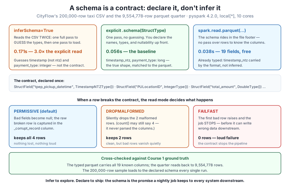
The Contract Enforces Itself: PERMISSIVE, DROPMALFORMED, FAILFAST#

Speed is the smaller half of the argument. The bigger half is what happens when the data arrives wrong — a column’s values drift, a row is truncated, a stray N/A lands where a number belongs. In an unattended job, this is not a hypothetical; it is Tuesday. An inferred schema has no opinion about correctness — it just re-guesses from whatever showed up, and if the new data guesses to a different type, downstream code breaks silently. An explicit schema turns that same event into a decision you made in advance, because the read mode governs what Spark does with a row that violates the declared shape.

To see all three modes, write a tiny malformed CSV by hand — two good rows, one with a non-numeric PULocationID, one with a missing column:

BAD = "c2m6l1_malformed.csv"
rows = [
    "tpep_pickup_datetime,PULocationID,total_amount",
    "2024-01-15 08:30:00,161,21.60",
    "2024-01-15 09:00:00,237,18.35",
    "2024-01-15 10:00:00,N/A,25.00",
    "2024-01-15 11:00:00,132",
]
with open(BAD, "w") as fh:
    fh.write("\n".join(rows) + "\n")

mini = StructType([
    StructField("tpep_pickup_datetime", TimestampNTZType(), True),
    StructField("PULocationID",         IntegerType(),      True),
    StructField("total_amount",         DoubleType(),       True),
])
mini_corrupt = StructType(mini.fields + [StructField("_corrupt_record", StringType(), True)])

permissive = (spark.read.schema(mini_corrupt)
    .option("header", "true")
    .option("mode", "PERMISSIVE")
    .option("columnNameOfCorruptRecord", "_corrupt_record")
    .csv(BAD))
permissive.show(truncate=False)

+--------------------+------------+------------+-----------------------------+
|tpep_pickup_datetime|PULocationID|total_amount|_corrupt_record              |
+--------------------+------------+------------+-----------------------------+
|2024-01-15 08:30:00 |161         |21.6        |NULL                         |
|2024-01-15 09:00:00 |237         |18.35       |NULL                         |
|2024-01-15 10:00:00 |NULL        |25.0        |2024-01-15 10:00:00,N/A,25.00|
|2024-01-15 11:00:00 |132         |NULL        |2024-01-15 11:00:00,132      |
+--------------------+------------+------------+-----------------------------+

PERMISSIVE is the default, and it is the forgiving one: it keeps every row, sets the fields it could not parse to NULL, and — because we added a _corrupt_record column and named it via columnNameOfCorruptRecord — it hands you the raw text of every row it couldn’t fully parse. Row three’s N/A became a NULL PULocationID; row four’s missing column became a NULL total_amount; and both broken rows are preserved verbatim in _corrupt_record so you can quarantine and inspect them later. Nothing is lost and nothing is loud — which is exactly right for a stage that wants to capture bad rows rather than crash, the pattern Lesson 2 builds on when it quarantines the strays.

DROPMALFORMED takes the opposite stance — throw the broken rows away and keep only what parses cleanly:

dropped = (spark.read.schema(mini).option("header", "true")
           .option("mode", "DROPMALFORMED").csv(BAD))
dropped.show(truncate=False)
print("rows kept (collect):", len(dropped.collect()))
print("rows via count()   :", dropped.count())

+--------------------+------------+------------+
|tpep_pickup_datetime|PULocationID|total_amount|
+--------------------+------------+------------+
|2024-01-15 08:30:00 |161         |21.6        |
|2024-01-15 09:00:00 |237         |18.35       |
+--------------------+------------+------------+
rows kept (collect): 2
rows via count()   : 4

show and collect agree: the two malformed rows are gone, 2 clean rows remain. But look at the honest surprise on the last line — count() returns 4, not 2. This is not a bug; it’s a lazy-evaluation subtlety worth internalizing. count() only needs to know how many rows there are, so Catalyst prunes the query down to counting lines and never actually parses the columns — and a row is only “malformed” once you try to parse the columns it violates. No parse, no drop, so count() sees all four lines. The lesson: DROPMALFORMED drops rows when the columns are read, and you cannot use a bare count() to trust that your data is clean. That gap between “counted” and “parsed” is precisely why the next mode exists.

FAILFAST is the strict one, and the right default for a production job that must never write wrong data: the first row that violates the schema raises an exception and stops everything.

try:
    (spark.read.schema(mini).option("header", "true")
        .option("mode", "FAILFAST").csv(BAD).collect())
    print("no error raised")
except Exception as err:
    for line in str(err).splitlines():
        if "Parse Mode: FAILFAST" in line:
            print("FAILFAST raised ->", line.strip())
            break

FAILFAST raised -> Parse Mode: FAILFAST. To process malformed records as null result, try setting the option 'mode' as 'PERMISSIVE'.  SQLSTATE: 22023

The read hit N/A in an integer column and threw — [MALFORMED_RECORD_IN_PARSING], parse mode FAILFAST. This is the contract enforcing itself in the loudest possible way: rather than silently null a value or quietly drop a row, the job halts before it can produce a corrupt result, so you find out at 2 a.m. from a failed run instead of at 9 a.m. from a wrong dashboard. Which mode you choose is a real engineering decision — PERMISSIVE to capture and quarantine, DROPMALFORMED to tolerate known noise, FAILFAST to guarantee correctness — but you can only make that decision because you declared a schema for the data to violate. Inference gives you nothing to enforce.

Clean up the scratch file and close the session:

import os
os.remove(BAD)
spark.stop()
print("session closed; scratch file removed")

session closed; scratch file removed

Practice Exercises#

Exercise 1 — Build the contract from the parquet. Instead of typing the ten StructFields by hand, derive them: read one month of parquet, grab .schema, and print it as a Python object with print(quarter.schema) (or, more readably, loop over quarter.schema.fields printing each field’s .name and .dataType). Now select just the ten columns the sample CSV uses and build a StructType from those fields. Read the CSV with your derived schema and confirm printSchema matches the hand-written taxi_schema from this lesson. Why is deriving the schema from a trusted parquet file a safer way to author the contract than typing it out?

Exercise 2 — Prove the extra pass with a bigger file. The 200,000-row timing was fast and a little noisy. Amplify it: read the full quarter as CSV is not available, so instead loop the sample read k times (say k=10) inside each timed function to make the per-call work bigger, and re-run the best_of comparison of explicit vs inferSchema=True. Does the ratio hold near 3x, grow, or shrink? Then explain, in one sentence each, why the explicit read scales with one pass while the inferred read scales with roughly two.

Exercise 3 — Design the mode for a real feed. You’re wiring the nightly taxi ingest. Write down, for each of these three requirements, which read mode you’d choose and one sentence of justification: (a) “the finance team must never see a total computed from a row we couldn’t parse”; (b) “we know ~0.1% of rows have a junk sensor field we don’t use, and we’d rather keep running than page someone”; (c) “we want to load everything and route the bad rows to a quarantine table for a human to review each morning.” Then, for requirement (c), sketch the two lines of PySpark that would split a PERMISSIVE read into clean rows and quarantined rows.

Summary#

A schema is the contract a production job keeps with its data: the declared names, types, and nullability that everything downstream depends on. This lesson drew the line between declaring that contract and inferring it. Reading CityFlow’s sample CSV with no schema gave ten string columns, because CSV is untyped text — useless for computation. Declaring the schema explicitly with StructType/StructField and applying it via .schema(...) produced the right types on read (timestamp_ntz for the pickup stamp, integer for PULocationID, double for total_amount) across all 200,000 rows. The alternative, inferSchema=True, cost a full extra pass over the file — 0.171s against the explicit read’s 0.056s, 3.0x slower — and guessed differently than the truth, typing the stamps as zone-aware timestamp and payment_type as integer where the contract wants timestamp_ntz and long. Parquet needed no pass at all: its 19-field schema came straight from the footer in 0.038s, already typed, and the quarter read back to Course 1’s exact 9,554,778 rows. Finally, the contract enforced itself on a malformed CSV through the read mode: PERMISSIVE nulled the bad fields and captured the raw rows in _corrupt_record (keeping all 4), DROPMALFORMED dropped the 2 broken rows (with the honest count()-says-4 subtlety), and FAILFAST raised and stopped the job. Speed is the smaller reason to declare a schema; controllable failure is the larger one.

Key Concepts#

• Schema as contract — the declared shape (names, types, nullability) of the data, written in code as a StructType. Production declares it so every run matches a known shape; ad-hoc work infers it because convenience beats rigor when nobody’s downstream.
• The inference pass — inferSchema=True reads the whole file once to guess types before loading it again, so it runs a full extra scan (measured here at 3.0x an explicit read) and can guess types that differ from the real contract. Parquet avoids this entirely by storing its schema in the file footer.
• StructType / StructField — the container and the column of an explicit schema; each StructField is a (name, type, nullable) triple. Apply the assembled StructType with .schema(...) on the reader, and confirm it with printSchema().
• timestamp_ntz — timestamp without time zone, a wall-clock instant in microseconds with no zone attached; it matches the taxi parquet and keeps a CSV read type-identical to the parquet, unlike inference’s zone-aware timestamp guess.
• Read modes — PERMISSIVE (default) nulls unparseable fields and can capture raw bad rows in _corrupt_record; DROPMALFORMED drops them (but a bare count() may not, since it never parses the columns); FAILFAST raises on the first violation. The mode is how the contract enforces itself.

Why This Matters#

The difference between a script and a pipeline is what happens when nobody is watching, and the schema is where that difference starts. A CityFlow ingest that infers its types is fast to write and slow to run — it pays a full extra scan of the data every night — but the real danger is silent: the day the source ships payment_type as a float, or the pickup column arrives in a different zone convention, inference simply re-guesses, and the wrong types flow downstream into a report that is subtly, unaccountably off. Declaring the schema turns that class of failure into a choice you already made: with FAILFAST the job stops loudly before it can write a wrong number; with PERMISSIVE and _corrupt_record the bad rows are captured for review instead of vanishing; with DROPMALFORMED known noise is tolerated without a 2 a.m. page. Every one of those is a deliberate posture toward bad data — and none of them is available to a job that never wrote its contract down. Reading a schema off the parquet footer showed the ideal: the shape travels with the data. When it can’t, you supply the shape yourself, once, and let it guard every run.

Continue Building Your Skills#

You now have the first discipline of a production ETL: the data’s shape is declared, not guessed, and the read mode decides what happens when a row breaks it. That contract is the foundation the rest of the module builds on. Lesson 2, Read, Clean, Transform, takes the explicitly-typed read you just wrote and makes it the first stage of a real pipeline — structured as reusable, tested functions rather than a session of ad-hoc calls. You’ll read the quarter with the schema from this lesson, then carry Course 1’s hard-won data-quality rules into a Spark cleaning stage: filter to the report window, preserve the negative-total accounting reversals that a careless filter would delete (dropping them adds $2.99M of phantom revenue), quarantine the stray timestamps into the very _corrupt_record-style bucket you met here, and key the zone join on the LocationID rather than the name. The schema was the promise; the clean stage is where the pipeline starts keeping it — and by the end of Lesson 2 the numbers will land back on the ground truth you already know: 9,554,757 trips kept, 21 quarantined, $256,692,373.14 in revenue.