Title here
Summary here
Lesson 1 gave you the first discipline of a production job: declare the schema, never infer it, so the read is a contract rather than a guess. You now have a StructType that describes every taxi column exactly. This lesson builds the body of the job that sits on top of that contract — the part that turns three raw Parquet files into CityFlow’s zone-hour analytics table — and it makes one architectural decision that every maintainable pipeline shares: the body is a few small functions, not one long chain of DataFrame calls.
That choice sounds like style, but it is the difference between a job you can trust at 3 a.m. and one you can only pray over. A single 40-line .filter().withColumn().join().groupBy() chain runs fine right up until the day a number looks wrong, and then you have nowhere to stand — no seam to inspect, no piece to test, no way to ask “is the cleaning wrong or the aggregation wrong?” without re-reading the whole thing. So we split the body into three functions with one job each: read_trips declares the schema and reads the months, clean_trips carries Course 1’s data-quality rules into Spark, and transform_to_report derives the hour, joins the zones, and aggregates. Each is independently runnable, and by the end of the lesson you will unit-test the cleaner on a four-row frame you build by hand — proving it drops a 2002 stray, keeps both halves of a reversal pair, and cancels them to exactly $40.00 — the kind of test a real job ships with. Every number lands on Course 1’s ground truth: 240,917 buckets, 9,554,757 trips, $256,692,373.14.
By the end of this lesson, you will be able to:
read_trips, clean_trips, transform_to_report — instead of one opaque method chaintotal_amount reversals fabricates $2,986,808.76 of revenue, rather than asserting itdate_trunc, broadcast-join the 265-row zone dimension on LocationID, and aggregate to the 240,917-bucket zone-hour reportassert unit test for clean_trips on a hand-built DataFrame — the payoff of the function structure, and the reason production code is written this wayYou’ll need pyspark with the JDK configured as in Module 1, Lesson 3, and the three taxi-quarter Parquet files plus taxi_zone_lookup.csv. Start the session.
Before we write a line of cleaning logic, look at the silhouette of what we are building. An ETL job’s body has exactly three moving parts, and naming them as functions makes the whole pipeline legible at a glance:
import warnings
warnings.filterwarnings("ignore")

from pyspark.sql import SparkSession, functions as F
from pyspark.sql.types import (StructType, StructField, IntegerType, LongType,
                               DoubleType, StringType, TimestampNTZType)

spark = (SparkSession.builder
         .appName("cityflow")
         .master("local[*]")
         .config("spark.ui.showConsoleProgress", "false")
         .getOrCreate())
spark.sparkContext.setLogLevel("ERROR")
Now the schema from Lesson 1 — the contract the read enforces. The taxi timestamps are timestamp_ntz (no zone), so we name TimestampNTZType; the ID and count columns are long/int, the money columns double:
TAXI_SCHEMA = StructType([
    StructField("VendorID", IntegerType(), True),
    StructField("tpep_pickup_datetime", TimestampNTZType(), True),
    StructField("tpep_dropoff_datetime", TimestampNTZType(), True),
    StructField("passenger_count", LongType(), True),
    StructField("trip_distance", DoubleType(), True),
    StructField("RatecodeID", LongType(), True),
    StructField("store_and_fwd_flag", StringType(), True),
    StructField("PULocationID", IntegerType(), True),
    StructField("DOLocationID", IntegerType(), True),
    StructField("payment_type", LongType(), True),
    StructField("fare_amount", DoubleType(), True),
    StructField("extra", DoubleType(), True),
    StructField("mta_tax", DoubleType(), True),
    StructField("tip_amount", DoubleType(), True),
    StructField("tolls_amount", DoubleType(), True),
    StructField("improvement_surcharge", DoubleType(), True),
    StructField("total_amount", DoubleType(), True),
    StructField("congestion_surcharge", DoubleType(), True),
    StructField("Airport_fee", DoubleType(), True),
])

QUARTER = ["yellow_tripdata_2024-01.parquet",
           "yellow_tripdata_2024-02.parquet",
           "yellow_tripdata_2024-03.parquet"]
That is the setup. The body itself is these three signatures, and you should read them before their bodies exist, because the shape is the lesson:
def read_trips(files, schema):
    """READ: one explicit-schema read of many files -> raw DataFrame."""
    return spark.read.schema(schema).parquet(*files)

def clean_trips(df):
    """CLEAN: window to the quarter, preserve reversals, flag, fill. No aggregation."""
    ...   # built up over the next three sections

def transform_to_report(df, zones):
    """TRANSFORM: derive the hour, join zones on ID, aggregate to zone-hour."""
    ...   # built at the end
Three functions, three verbs, one responsibility each. read_trips knows about files and schemas and nothing about cleaning. clean_trips takes any trips DataFrame and returns a cleaned one — it never mentions a file path, which is exactly why we will be able to hand it a four-row frame later and test it in a second. transform_to_report takes clean trips and the zone dimension and produces the report. Contrast this with the one-chain alternative: read.schema(...).parquet(...).filter(...).withColumn(...).na.fill(...).join(...).groupBy(...).agg(...). That chain computes the same answer, but it has no seams — you cannot run the cleaning without also running the read and the join, cannot assert on the cleaner’s output, cannot reuse the cleaning in a second job that aggregates differently. The functions are the same work, cut where a test can reach. Let’s fill them in, measuring as we go.
read_trips is the whole READ stage, and it is deliberately tiny. spark.read.schema(schema).parquet(*files) reads all three months as one logical DataFrame under the declared contract — no inference pass, no per-file schema drift. Call it and confirm the shape:
raw = read_trips(QUARTER, TAXI_SCHEMA)

print("columns          :", len(raw.columns))
print("read partitions  :", raw.rdd.getNumPartitions())
print("raw quarter rows :", f"{raw.count():,}")
columns : 19
read partitions : 10
raw quarter rows : 9,554,7789,554,778 raw rows across the quarter — Jan + Feb + Mar 2024 — planned into 10 partitions (Spark matches the read to this machine’s 10 cores, as Module 2 measured; the three-file count is the same 10 a single month gets). This is the number every later stage is measured against. It is also dirty: it still contains out-of-quarter strays, reversals, a broken odometer, and three quarters of a million rows with missing metadata. READ’s only job is to get the bytes in under a known schema; it judges nothing. Everything that follows is clean_trips.
Course 1’s golden rule opens every report: restrict the data to the quarter you actually mean — pickups on or after 2024-01-01 and strictly before 2024-04-01 — before you count anything. This is not arithmetic bookkeeping; it is a data-integrity filter, because the monthly files carry a few rows whose timestamps are simply wrong. Measure what it removes:
window = ((F.col("tpep_pickup_datetime") >= "2024-01-01") &
          (F.col("tpep_pickup_datetime") <  "2024-04-01"))

kept = raw.filter(window).count()
print(f"raw quarter rows      : {raw.count():,}")
print(f"after the window       : {kept:,}")
print(f"quarantined by window  : {raw.count() - kept:,}")
raw quarter rows : 9,554,778
after the window : 9,554,757
quarantined by window : 21Exactly 21 rows quarantined, leaving 9,554,757 — Course 1’s verified kept-count, reproduced on the first try. These 21 are not near-boundary spill; they are wild. The deepest of them, as Module 3’s cleaning lesson surfaced, is a pickup stamped 2002-12-31 22:17:10 hiding in the March file — a meter clock that was never set. Removing these is the one delete in the whole cleaner that is unambiguously right, because we are not judging the rows bad, we are defining the population the report is about. Every other decision in clean_trips is the opposite: keep the row, add knowledge. That is the stage-one line of the function:
# clean_trips, stage 1 - the window (the only justified delete)
in_quarter = raw.filter(window)
print("stage 1 rows:", f"{in_quarter.count():,}")
stage 1 rows: 9,554,757Here is the stage that separates a correct cleaner from a plausible-looking one. Some trips have a negative total_amount, and the untrained reflex is filter(total_amount >= 0) — negative money “looks wrong.” Count them first, then prove with a SUM why the reflex is the bug. The measurement is the point; we do not assert the reversals are safe, we measure the damage of dropping them:
neg = in_quarter.filter(F.col("total_amount") < 0).count()

rev_keep = in_quarter.agg(F.sum("total_amount")).first()[0]
rev_drop = (in_quarter.filter(F.col("total_amount") >= 0)
                      .agg(F.sum("total_amount")).first()[0])

print(f"negative-total rows           : {neg:,}")
print(f"revenue KEEPING the reversals : ${rev_keep:,.2f}")
print(f"revenue DROPPING the reversals: ${rev_drop:,.2f}")
print(f"phantom revenue introduced    : ${rev_drop - rev_keep:,.2f}")
negative-total rows : 115,894
revenue KEEPING the reversals : $256,692,373.14
revenue DROPPING the reversals: $259,679,181.90
phantom revenue introduced : $2,986,808.76115,894 negative rows — over one percent of the quarter, far too many and too systematic to be random errors. They are reversals: a charge billed, voided, and usually re-billed. The vendor leaves both the original and its offsetting entry in the ledger on purpose, and total_amount is designed so SUM lets each pair cancel. Keeping them sums to $256,692,373.14 — Course 1 to the cent. Dropping them reports $259,679,181.90, inventing $2,986,808.76 of revenue CityFlow never earned, because the filter removes each reversal while leaving its erroneous original behind with nothing to cancel it. This is the number that justifies the whole “clean is restraint, not deletion” philosophy of the module: a one-line filter that felt like hygiene fabricated nearly three million dollars. So clean_trips does nothing to the negatives at all — the correct cleaning of a reversal is the window filter it already passed:
# clean_trips, stage 2 - reversals: PRESERVE (the correct action is no action)
preserved = in_quarter   # the 115,894 negatives stay; SUM will cancel the pairs
Why this belongs in a tested function, not a chain
The reversal trap is invisible in a method chain — filter(total_amount >= 0) reads like ordinary hygiene and slips through code review. Isolated in clean_trips, it becomes something you can pin down with a test: feed the function a known reversal pair and assert the sum is zero, not the positive half. A bug that hides in a 40-line chain becomes a one-line failing assertion in a 4-line function. That is not a stylistic win — it is the difference between catching the $2,986,808.76 error in a unit test and shipping it to a dashboard.
Not every strange value is secretly correct. trip_distance really does contain nonsense — but the response is still not deletion. Find the maximum, then label rather than remove:
mx = preserved.agg(F.max("trip_distance")).first()[0]
print(f"max trip_distance: {mx:,.1f} miles")
max trip_distance: 312,722.3 miles312,722.3 miles in a five-borough taxi is a broken odometer — genuinely wrong, unlike the reversals. But filter(trip_distance < 100) would also delete the 215,764 legitimate zero-mile records (curbside cancellations, minimum-charge waits) that some downstream question needs. So we flag with when/otherwise, adding a column instead of removing rows. And the metadata nulls get filled, not dropped: an audit shows five columns share the identical null count, and they are co-located in the same rows — complete trips with lean metadata, not missing trips:
# audit which columns are actually null (never guess before cleaning)
exprs = [F.sum(F.col(c).isNull().cast("int")).alias(c) for c in raw.columns]
audit = preserved.agg(*exprs).first().asDict()
print("columns with nulls:", {c: f"{n:,}" for c, n in audit.items() if n > 0})
columns with nulls: {'passenger_count': '751,962', 'RatecodeID': '751,962', 'store_and_fwd_flag': '751,962', 'congestion_surcharge': '751,962', 'Airport_fee': '751,962'}Five columns, all 751,962 — a signature, not a coincidence. A blanket na.drop() would delete every one of those real trips (a 7.9% undercount); na.fill keeps the trip and marks the gap. Now assemble all three stages into the finished clean_trips — one function, four transformations, zero surprises:
def clean_trips(df):
    window = ((F.col("tpep_pickup_datetime") >= "2024-01-01") &
              (F.col("tpep_pickup_datetime") <  "2024-04-01"))
    return (df
            .filter(window)                                   # 1: window - the only delete
            .withColumn("distance_flag",                      # 2: flag dirt, keep the row
                F.when(F.col("trip_distance") > 100, "suspect")
                 .when(F.col("trip_distance") == 0, "zero")
                 .otherwise("ok"))
            .na.fill({"passenger_count": 0, "RatecodeID": 99, # 3: fill metadata nulls
                      "congestion_surcharge": 0.0, "Airport_fee": 0.0}))
            # reversals are PRESERVED by omission - no filter touches total_amount
Run it on the real quarter and confirm the count and the distance flags in one pass:
cleaned = clean_trips(raw)
print("cleaned rows:", f"{cleaned.count():,}")
cleaned.groupBy("distance_flag").count().orderBy("distance_flag").show()
cleaned rows: 9,554,757
+-------------+-------+
|distance_flag| count|
+-------------+-------+
| ok|9338741|
| suspect| 252|
| zero| 215764|
+-------------+-------+9,554,757 trips survive — every reversal, every zero-mile record, every lean-metadata trip. The 252 suspect and 215,764 zero distances are labelled, not gone. clean_trips deleted exactly the 21 rows the window quarantined and not one more. That restraint is what makes the next stage’s numbers match Course 1.
transform_to_report turns clean trips into the analytics table. Three moves: derive the pickup hour so trips bucket by time, attach zone names so 132 becomes “JFK Airport”, and aggregate. The hour comes from date_trunc, which floors a timestamp to the hour boundary — no UDF, a built-in that pushes into the plan:
def transform_to_report(df, zones):
    hourly = df.withColumn("pickup_hour",
                           F.date_trunc("hour", "tpep_pickup_datetime"))
    named = hourly.join(F.broadcast(zones),
                        hourly.PULocationID == zones.LocationID, "left")
    return (named.groupBy("PULocationID", "Zone", "Borough", "pickup_hour")
                 .agg(F.count(F.lit(1)).alias("trips"),
                      F.round(F.sum("total_amount"), 2).alias("revenue")))
Two design decisions carry the module’s discipline. First, F.broadcast(zones) ships the tiny 265-row dimension to every task instead of shuffling nine million trips — a BroadcastHashJoin, the pattern Module 3’s joins lesson measured (Spark would auto-broadcast a table this small anyway; naming it makes the intent explicit and the plan stable). Second, we key on LocationID, never the zone name — there are two zones both named “Corona” (IDs 56 and 57), so grouping by name would silently merge them; grouping by ID keeps them apart and carries the name only for display. Load the zone dimension (casting its LocationID from the CSV’s string to an int so the join keys match) and build the report:
zones = (spark.read.option("header", True).csv("taxi_zone_lookup.csv")
              .withColumn("LocationID", F.col("LocationID").cast("int")))

report = transform_to_report(cleaned, zones)
print("zone-hour buckets:", f"{report.count():,}")
zone-hour buckets: 240,917240,917 buckets — one row per (zone, pickup-hour) pair, Course 1’s exact bucket count. This groupBy is the module’s canonical shuffle; AQE coalesces its 200 configured post-shuffle partitions down to 6 to fit the data, as Module 4 showed. The table is now the shape a dashboard consumes: zone, hour, trips, revenue.
The whole point of three functions is that the pipeline is now one legible line — read, clean, transform — and every intermediate is inspectable. Run the composition end to end and cross-check all three ground-truth numbers at once:
pipeline = transform_to_report(clean_trips(read_trips(QUARTER, TAXI_SCHEMA)), zones)

totals = pipeline.agg(F.count(F.lit(1)).alias("buckets"),
                      F.sum("trips").alias("trips"),
                      F.sum("revenue").alias("revenue")).first()

print(f"buckets : {totals['buckets']:,}")
print(f"trips   : {totals['trips']:,}")
print(f"revenue : ${totals['revenue']:,.2f}")
buckets : 240,917
trips : 9,554,757
revenue : $256,692,373.14Three numbers, three matches: 240,917 buckets, 9,554,757 trips, $256,692,373.14 — Course 1 to the cent, produced by a Spark job assembled from three independently-testable functions. Nothing was thrown away that shouldn’t be, and the reversals cancelled exactly as the ledger intended. The podium confirms the shape of the answer, not just its totals:
podium = (pipeline.groupBy("PULocationID", "Zone")
                  .agg(F.sum("trips").alias("total_trips"))
                  .orderBy(F.col("total_trips").desc()))
podium.show(5, truncate=False)
+------------+---------------------+-----------+
|PULocationID|Zone |total_trips|
+------------+---------------------+-----------+
|161 |Midtown Center |453825 |
|237 |Upper East Side South|439138 |
|132 |JFK Airport |429745 |
|236 |Upper East Side North|416508 |
|162 |Midtown East |336460 |
+------------+---------------------+-----------+
only showing top 5 rowsMidtown Center leads at 453,825 trips, then Upper East Side South (439,138), JFK (429,745), Upper East Side North (416,508), and Midtown East (336,460) — Course 1’s busiest-zone ranking, reproduced. JFK riding third is the airport hot-key that later modules will watch as a skew source.
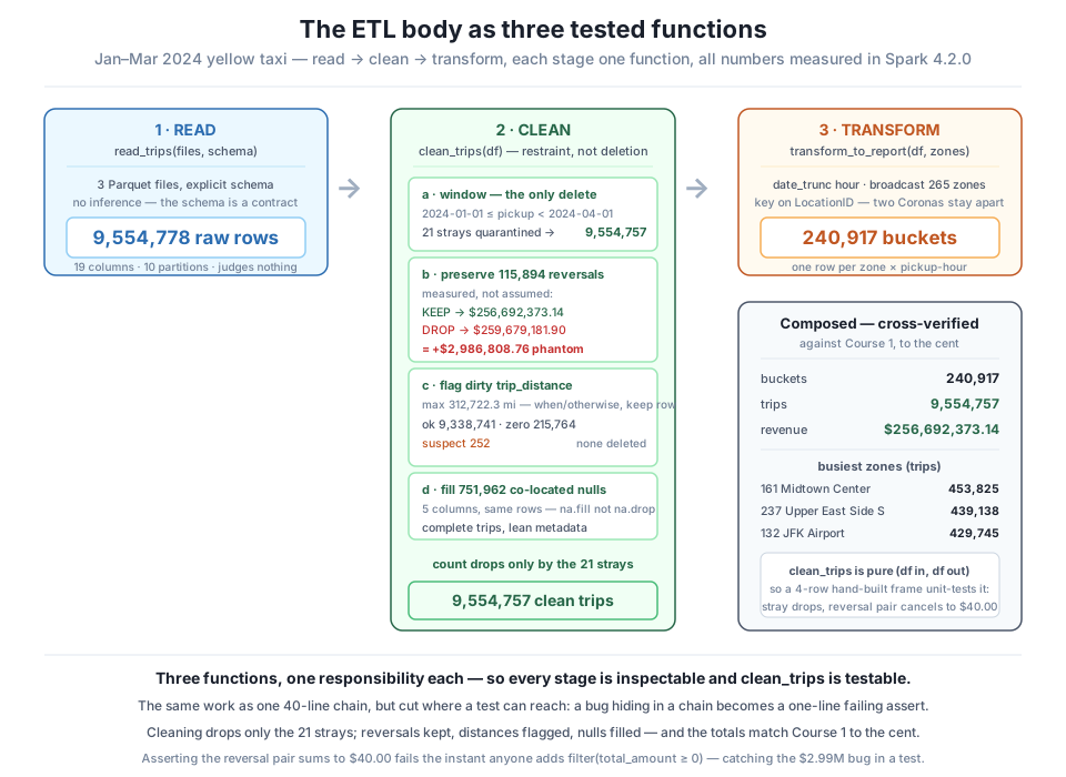
read_trips reads 9,554,778 raw rows under the explicit schema; clean_trips windows to 9,554,757 (the only delete is 21 strays), preserves the 115,894 reversals because dropping them invents $2,986,808.76, flags the 312,722.3-mile trip_distance, and fills 751,962 co-located nulls; transform_to_report derives the hour with date_trunc, broadcast-joins the 265 zones on LocationID, and aggregates to 240,917 buckets. Composed, they land on Course 1 to the cent: 240,917 / 9,554,757 / $256,692,373.14, Midtown Center leading at 453,825 trips.clean_tripsEverything so far argued that the three-function shape enables testing. Now collect on that promise. Because clean_trips takes any trips DataFrame and mentions no file path, we can hand it a four-row frame we build by hand — one reversal pair, one out-of-window stray, one dirty-distance-with-null row — and assert exactly what the cleaner should do, in under a second, with no Parquet and no pytest. This is the test a real job ships with:
from pyspark.sql import Row
import datetime as dt

def test_clean_trips():
    tiny = spark.createDataFrame([
        # a reversal PAIR, both in-window - must both survive and cancel
        Row(tpep_pickup_datetime=dt.datetime(2024, 2, 10, 9, 30), trip_distance=2.0,
            passenger_count=1, RatecodeID=1, congestion_surcharge=2.5,
            Airport_fee=0.0, total_amount=18.50,  PULocationID=161),
        Row(tpep_pickup_datetime=dt.datetime(2024, 2, 10, 9, 35), trip_distance=2.0,
            passenger_count=1, RatecodeID=1, congestion_surcharge=2.5,
            Airport_fee=0.0, total_amount=-18.50, PULocationID=161),
        # an OUT-OF-WINDOW stray (2002) - must be dropped
        Row(tpep_pickup_datetime=dt.datetime(2002, 12, 31, 22, 17, 10), trip_distance=1.0,
            passenger_count=1, RatecodeID=1, congestion_surcharge=0.0,
            Airport_fee=0.0, total_amount=18.0,   PULocationID=50),
        # dirty distance + null metadata - flag + fill, never drop
        Row(tpep_pickup_datetime=dt.datetime(2024, 3, 1, 0, 0, 0), trip_distance=312722.3,
            passenger_count=None, RatecodeID=None, congestion_surcharge=None,
            Airport_fee=None, total_amount=40.0,  PULocationID=132),
    ])

    out = clean_trips(tiny)
    got = {r.PULocationID: r for r in out.collect()}
    revenue = out.agg(F.sum("total_amount")).first()[0]

    assert out.count() == 3,                 "the 2002 stray must be dropped"
    assert 50 not in got,                    "the out-of-window pickup should be gone"
    assert abs(revenue - 40.0) < 1e-6,       "reversal pair must cancel: 18.5 + (-18.5) + 40 = 40"
    assert got[132].distance_flag == "suspect", "312,722 mi must be flagged, not deleted"
    assert got[132].passenger_count == 0,    "null metadata must be filled, not dropped"
    print("all 5 assertions passed - clean_trips behaves exactly as specified")

test_clean_trips()
all 5 assertions passed - clean_trips behaves exactly as specifiedRead what those five assertions pin down, because together they are the entire cleaning contract on four rows. The count drops from four to three — the 2002 stray is gone, and only it. The revenue sums to exactly $40.00, not $58.50: the reversal pair ($18.50 and −$18.50) cancelled, proving the pipeline preserves reversals rather than dropping the negative half. The broken 312,722-mile row is present with distance_flag = "suspect", flagged not deleted. And its null passenger_count came back as 0, filled not dropped. If a future edit ever “cleans up” clean_trips by adding filter(total_amount >= 0), this test fails on the revenue assertion in under a second — the $2,986,808.76 bug caught before it can reach a single row of production data. That is what the function structure buys you: not tidier code, but a place to stand a test that guards the exact mistake this module exists to prevent.
A hand-built frame is a real fixture
spark.createDataFrame([Row(...), ...]) builds a DataFrame from Python objects with no file at all — the fastest fixture in Spark. Because clean_trips is pure with respect to its input (a DataFrame in, a DataFrame out, no path, no global state), the four-row frame exercises the identical code path the nine-million-row quarter does. That is the deep reason to split the body into functions: a stage you can call with hand-made input is a stage you can test, and a stage you can test is a stage you can trust to run unattended tonight.
One session, one shutdown — release it now that every stage is built, composed, and tested:
spark.stop()
print("session stopped")
session stoppedExercise 1 — Split clean_trips and test each half. The cleaner does two conceptually different jobs: scoping (the window delete) and repairing (flag + fill, which never change the row count). Refactor it into window_trips(df) and repair_trips(df) so clean_trips(df) becomes repair_trips(window_trips(df)). Then write two separate assert tests on hand-built frames: one proving window_trips drops an out-of-quarter row and keeps an in-quarter one, and one proving repair_trips never changes the row count (it only adds distance_flag and fills nulls). Confirm the composed function still produces 9,554,757 rows on the real quarter.
Hint
repair_trips should assert out.count() == df.count() on its fixture — the whole point of separating it is that repair is count-preserving, so a test that fails when the count changes will catch anyone who later slips a filter into the repair stage. Build the window_trips fixture with one row dated 2024-02-15 and one dated 2023-12-31; expect the second to vanish. Keep the money and location columns present in both fixture rows or the schema inference on the tiny frame will complain.
Exercise 2 — Parameterize the window. Right now the quarter dates are hard-coded inside clean_trips. Give it the signature clean_trips(df, start="2024-01-01", end="2024-04-01") so the same function can clean any period. Run it with start="2024-02-01", end="2024-03-01" to clean just February, count the result, and cross-check against Course 1’s February figure. Then write an assert-test on a hand-built frame proving that a row on the end boundary is excluded (the window is < end, not <= end).
Hint
February alone should keep close to Course 1’s Feb count (the raw Feb file is 3,007,526 rows, minus its own out-of-month strays). The boundary test is the subtle one: create a row stamped exactly 2024-03-01 00:00:00 and assert it is dropped when end="2024-03-01", because pickup < end is strict — this is exactly why the quarter window uses < "2024-04-01" and not <= "2024-03-31", which would miss the last day’s final hours.
Exercise 3 — Add a transform-stage test. transform_to_report also deserves a unit test. Build a tiny zones frame with two rows both named "Corona" but with different LocationIDs (56 and 57), plus a couple of trips keyed to each. Run transform_to_report and assert that the two Coronas stay separate in the output (two distinct PULocationID groups), proving the key-on-ID discipline. Then, as a contrast, group your trips by Zone name instead of ID and show the two Coronas collapse into one — the bug the ID key prevents.
Hint
The assertion is on distinct PULocationID values in the report: with two Coronas keyed on ID you should see both 56 and 57; grouping by the Zone string collapses them to a single “Corona” row that sums trips from both real zones. This is the same corruption dropping the reversals caused, wearing a different hat — a join or group on a non-unique attribute silently merges records that a unique key would keep apart. date_trunc("hour", ...) on your fixture timestamps will bucket by hour, so keep the fixture pickups within one hour if you want a single bucket per zone.
A production ETL body is not one long method chain — it is a few small functions, each doing one stage and each testable in isolation, and this lesson built CityFlow’s quarterly report in exactly that shape. read_trips(files, schema) reads the three months under Lesson 1’s explicit schema to 9,554,778 raw rows across 10 partitions, judging nothing. clean_trips(df) carries Course 1’s rules into Spark: the quarter window is the only delete, quarantining exactly 21 strays to 9,554,757 kept; the 115,894 negative-total_amount reversals are preserved, because we measured — not assumed — that dropping them fabricates $2,986,808.76 of phantom revenue ($259,679,181.90 vs the true $256,692,373.14); the 312,722.3-mile trip_distance is flagged with when/otherwise (252 suspect, 215,764 zero, 9,338,741 ok) rather than deleted; and the 751,962 co-located metadata nulls across five columns are filled, not dropped. transform_to_report(df, zones) derives the pickup hour with date_trunc, broadcast-joins the 265-row zone dimension on LocationID (keeping the two Coronas apart), and aggregates to 240,917 zone-hour buckets. Composed, the three functions reproduce Course 1 to the cent — 240,917 / 9,554,757 / $256,692,373.14, Midtown Center leading at 453,825 trips — and, because clean_trips mentions no file path, a four-row hand-built frame unit-tests it in under a second: the stray drops, the reversal pair cancels to exactly $40.00, the dirty distance is flagged, the null is filled.
read_trips / clean_trips / transform_to_report, one responsibility each, cut the ETL body where a test can reach; the same work as a 40-line chain, but with seams you can inspect and assert on.date_trunc + broadcast join on ID — derive the hour with a built-in (no UDF), ship the 265-row zone dimension with F.broadcast, and key on LocationID so the two “Corona” zones never merge — the aggregate lands on 240,917 buckets.clean_trips takes a DataFrame and no path, spark.createDataFrame([Row(...)]) builds a fixture that exercises the identical code path as the 9.5M-row quarter, testable with plain assert and no pytest.filter(total_amount >= 0) into the cleaner, catching the $2,986,808.76 error in a unit test instead of on a dashboard.The reason production code is written as small functions is not neatness — it is that a job which runs unattended every night must be trustable without being watched, and you cannot trust what you cannot test. A monolithic read-clean-transform chain computes the right answer today and gives you no way to prove it will tomorrow, after the next engineer “tidies” it. Split into read_trips, clean_trips, and transform_to_report, the same pipeline becomes a set of claims you can check: the cleaner drops exactly the strays and preserves the reversals, the transform keys on ID and lands on 240,917 buckets, and each claim is a four-row test that runs in a second. This is the shape every later module builds on — Lesson 3 will make transform_to_report’s output durable by writing it to a partitioned Parquet table, Lesson 4 will make the whole job idempotent so a re-run never double-counts, and the guided project will assemble all of it into one script an orchestrator can schedule. The functions you wrote here are the units that get written, partitioned, and re-run. A pipeline you can trust to run tonight is a pipeline whose every stage you could hand a fistful of rows and predict the answer — and that is exactly what you just did.
You now have the ETL body as three tested functions, and a report that matches Course 1 to the cent — but that report lives only in memory. The moment spark.stop() runs, the 240,917 buckets vanish, and a job whose output disappears when the session ends is not yet a production job. Lesson 3, Writing Results, makes the report durable: you’ll df.write the zone-hour table to Parquet, choose a mode (overwrite, append, error, ignore) deliberately rather than by default, and — the lesson’s measured payoff — partitionBy a column like pickup date or borough so that a later read with a matching filter prunes to a handful of files instead of scanning the whole table, the same clustering win Course 1 proved for out-of-core reads, now in Spark’s write form. You’ll also meet the small-files problem and the coalesce/repartition dials that control it. The body is built and tested; next you give its output a home on disk that later reads can navigate quickly.
Keep DATATWEETS free. Help fund practical data, AI, and engineering lessons for learners worldwide.
