Title here
Summary here
Lesson 2 built the body of CityFlow’s job as three tested functions — read with an explicit schema, clean while preserving the accounting reversals, transform into the zone-hour shape — and cross-checked the result against Course 1’s ground truth: 9,554,757 trips kept, 21 quarantined, $256,692,373.14 in revenue. But so far that result has only ever lived in memory. A production ETL is not a query you watch return; it is a job that writes something other systems read tomorrow morning. This lesson is the write, and it is not the throwaway .save() it looks like. How you lay the output down decides how fast every downstream query runs, how many files pile up, and whether a re-run corrupts the table or replaces it cleanly.
The engine you tuned in Modules 4 and 5 already taught the punchline. In Catalyst’s Optimizations you saw that the raw TLC file ships no row-group statistics, so a pushed filter skipped nothing — and that writing your own partitionBy copy turned the same filter into a directory decision that skipped 95% of the data. That was a read-side experiment on a throwaway file. Now it becomes the write side of a real analytics table. You’ll write CityFlow’s cleaned trips partitioned by pickup date, read one day back, and measure exactly what the layout buys: 2 files and 77,033 rows touched instead of the flat table’s 10 files and 140,000-to-560,000 rows — and you’ll see, honestly, why the flat number swings so wildly and why partitioning is the only version that comes with a guarantee.
By the end of this lesson, you will be able to:
df.write.format("parquet").mode(...).save(path) and predict what each of the four save modes — overwrite, append, ignore, error — does when the path already existspartitionBy("pickup_date") and read its on-disk col=value/ layout and _SUCCESS markerPartitionFilters open 1 directory of 91 (2 files, 77,033 rows) instead of the flat table’s full scanrepartition and coalesce, trading a shuffle for one file per partition instead of 176 scattered onesmode("overwrite") to rebuild a partitioned table — the write pattern the next lesson makes idempotentYou’ll need pyspark and pyarrow. Let’s write some Parquet.
Every write in Spark is the same three-part sentence: df.write starts a writer, .format(...) / .mode(...) / .option(...) configure it, and a terminal .save(path) (or a format shortcut like .parquet(path)) triggers the job. The default format is Parquet — columnar (stored column-by-column, so a reader touches only the columns it needs), typed (the schema travels inside the file, no inference on read), and compressed (Snappy by default). It is the format you want for an analytics table, and everything in this lesson writes it.
The one parameter that will bite you if you ignore it is mode: it decides what happens when the output path already exists, which for a nightly job is every night after the first. There are four. Start the session and watch the default, overwrite.
import warnings
warnings.filterwarnings("ignore")
import os, time, shutil, glob, subprocess
from pyspark.sql import SparkSession
from pyspark.sql import functions as F

spark = (SparkSession.builder
         .appName("cityflow")
         .master("local[*]")
         .config("spark.ui.showConsoleProgress", "false")
         .getOrCreate())
spark.sparkContext.setLogLevel("ERROR")

demo = spark.range(0, 5).withColumn("v", F.col("id") * 10)
MODES = "c2m6l3_modes.parquet"
if os.path.exists(MODES):
    shutil.rmtree(MODES)

demo.write.format("parquet").mode("overwrite").save(MODES)
kept = [f for f in sorted(os.listdir(MODES)) if not f.startswith(".")]
print("after overwrite, directory holds:", kept)
print("rows on disk:", spark.read.parquet(MODES).count())
after overwrite, directory holds: ['_SUCCESS', 'part-00000-....snappy.parquet', 'part-00001-....snappy.parquet', 'part-00003-....snappy.parquet', 'part-00005-....snappy.parquet', 'part-00007-....snappy.parquet', 'part-00009-....snappy.parquet']
rows on disk: 5(The part-* filenames carry a run-specific UUID, shortened to ... here.) The first thing to notice is that save(path) writes a directory, not a file. Spark is a parallel engine: each task writes its own part-NNNNN file, and a five-row DataFrame with the default parallelism produced several of them. The second thing is the last entry: _SUCCESS. Spark writes every part-* file first, and only when all of them have committed does it drop this empty marker. Its presence is the atomic signal every downstream consumer should check — _SUCCESS means the job finished; no _SUCCESS means a partial, untrustworthy write. A job that died halfway leaves part-* files but no marker, and a careful reader treats that directory as absent.
Now the other three modes, against a path that already exists.
demo.write.mode("append").parquet(MODES)
print("append  -> rows:", spark.read.parquet(MODES).count())

spark.range(100, 103).write.mode("ignore").parquet(MODES)
print("ignore  -> rows:", spark.read.parquet(MODES).count(), "(path existed, write skipped)")

try:
    demo.write.mode("error").parquet(MODES)
except Exception as e:
    print("error   -> raised", type(e).__name__, "(path exists)")

demo.write.mode("overwrite").parquet(MODES)
print("overwrite -> rows:", spark.read.parquet(MODES).count(), "(replaced)")
append -> rows: 10
ignore -> rows: 10 (path existed, write skipped)
error -> raised AnalysisException (path exists)
overwrite -> rows: 5 (replaced)Four different answers to “the path is already here”:
append adds new part-* files alongside the old ones — 5 rows became 10. This is the mode that silently double-counts a re-run, the trap Lesson 4 exists to close.ignore is a no-op if the path exists: the 3 rows we tried to write were skipped, the count stayed at 10. “Leave whatever is already there.”error (also spelled errorifexists, and the true default for save() when you name no mode) refuses and raises AnalysisException. Fail rather than touch existing data.overwrite replaces the directory’s contents entirely — back to the original 5 rows.For a rebuildable analytics table, overwrite is almost always the right choice, and the rest of this lesson uses it. Keep append in view as the one to distrust.
Now the real output. We rebuild CityFlow’s cleaned trips exactly as Lesson 2 did — window to the quarter, keep the columns the analytics table needs — and add one derived column that will become the partition key: pickup_date, the calendar day of each trip. A partition key should be a column downstream queries filter on constantly and whose cardinality is modest; a dashboard that asks “what happened on the 15th?” makes the date exactly that.
FILES = ["yellow_tripdata_2024-01.parquet",
         "yellow_tripdata_2024-02.parquet",
         "yellow_tripdata_2024-03.parquet"]
LO, HI = "2024-01-01", "2024-04-01"

trips = (spark.read.parquet(*FILES)
    .where((F.col("tpep_pickup_datetime") >= F.lit(LO)) &
           (F.col("tpep_pickup_datetime") <  F.lit(HI)))
    .withColumn("pickup_date", F.to_date("tpep_pickup_datetime"))
    .withColumn("pickup_hour", F.date_trunc("hour", "tpep_pickup_datetime"))
    .select("pickup_date", "pickup_hour", "PULocationID", "total_amount"))
trips.cache()

n_rows = trips.count()
revenue = trips.agg(F.round(F.sum("total_amount"), 2)).first()[0]
n_dates = trips.select("pickup_date").distinct().count()
print(f"cleaned rows : {n_rows:,}")
print(f"revenue      : {revenue:,.2f}")
print(f"distinct days: {n_dates}")
cleaned rows : 9,554,757
revenue : 256,692,373.14
distinct days: 91The cross-check holds — 9,554,757 rows and $256,692,373.14, the same numbers Lesson 2 wrote and Course 1 pinned — and the quarter spans 91 calendar days (Jan + Feb + Mar 2024). We cache() the table because every write and read below reuses it, and re-deriving it each time would waste the whole lesson’s runtime. First, write it the naive way: flat, unpartitioned.
def files_under(path):
    return len(glob.glob(os.path.join(path, "**", "*.parquet"), recursive=True))

FLAT = "c2m6l3_trips_flat.parquet"
if os.path.exists(FLAT):
    shutil.rmtree(FLAT)

t = time.perf_counter()
trips.write.format("parquet").mode("overwrite").save(FLAT)
print(f"wrote {FLAT} in {time.perf_counter()-t:.1f}s")
print("part files      :", files_under(FLAT))
print("_SUCCESS marker :", os.path.exists(os.path.join(FLAT, "_SUCCESS")))
print("sample entries  :", [f for f in sorted(os.listdir(FLAT)) if not f.startswith(".")][:3], "...")
wrote c2m6l3_trips_flat.parquet in 3.6s
part files : 10
_SUCCESS marker : True
sample entries : ['_SUCCESS', 'part-00000-....snappy.parquet', 'part-00001-....snappy.parquet'] ...Ten part-* files — one per input partition (the quarter reads as 10 partitions, as Module 1 established) — and a _SUCCESS marker. Every trip lives somewhere in those ten files, in whatever order Spark read them. Now the same data, partitioned by day.
PART = "c2m6l3_trips_by_date.parquet"
if os.path.exists(PART):
    shutil.rmtree(PART)

t = time.perf_counter()
trips.write.partitionBy("pickup_date").mode("overwrite").parquet(PART)
print(f"wrote {PART} in {time.perf_counter()-t:.1f}s")

part_dirs = sorted(d for d in os.listdir(PART) if d.startswith("pickup_date="))
print("partition directories:", len(part_dirs))
print("first three          :", part_dirs[:3])
print("total files written  :", files_under(PART))
print("files in one day dir :", files_under(os.path.join(PART, "pickup_date=2024-01-15")))
wrote c2m6l3_trips_by_date.parquet in 6.6s
partition directories: 91
first three : ['pickup_date=2024-01-01', 'pickup_date=2024-01-02', 'pickup_date=2024-01-03']
total files written : 176
files in one day dir : 2The single call partitionBy("pickup_date") reshaped the whole output. Instead of ten files in one directory, there are now 91 sub-directories, one per day, each named pickup_date=2024-01-01 — the column and its value baked into the path. This is the crucial move: the value 2024-01-15 no longer lives only inside the files; it is the directory. A reader can decide whether a day is relevant by looking at a folder name, before opening a single Parquet footer. Notice the column also vanished from the data files themselves — Spark stores a partition column only in the path, and reconstructs it on read. (Set that aside for now: 176 total files across 91 days, roughly two per day, is a number we’ll come back to.)
Here is the whole reason to partition. CityFlow’s dashboard asks about one day at a time. Filter the partitioned table to January 15th and read the physical plan.
DAY = "2024-01-15"
p_read = spark.read.parquet(PART).where(F.col("pickup_date") == DAY)
print("=== partitioned read plan ===")
p_read.explain()
=== partitioned read plan ===
== Physical Plan ==
*(1) ColumnarToRow
+- FileScan parquet [pickup_hour#661,PULocationID#662,total_amount#663,pickup_date#664] Batched: true, DataFilters: [], Format: Parquet, Location: InMemoryFileIndex(1 paths)[...], PartitionFilters: [isnotnull(pickup_date#664), (pickup_date#664 = 2024-01-15)], PushedFilters: [], ReadSchema: struct<pickup_hour:timestamp,PULocationID:int,total_amount:double>(The Location path is shortened to [...] — it was the absolute work-directory path.) Read it exactly as the Catalyst lesson taught. The filter landed in PartitionFilters: [isnotnull(pickup_date), (pickup_date = 2024-01-15)], PushedFilters is empty, and Location reports InMemoryFileIndex(1 paths) — one path, the single directory pickup_date=2024-01-15, resolved at planning time. Spark decided which of the 91 folders to open before touching data. Now the flat table, same filter.
f_read = spark.read.parquet(FLAT).where(F.col("pickup_date") == DAY)
print("=== flat read plan ===")
f_read.explain()
=== flat read plan ===
== Physical Plan ==
*(1) Filter (isnotnull(pickup_date#666) AND (pickup_date#666 = 2024-01-15))
+- *(1) ColumnarToRow
+- FileScan parquet [pickup_date#666,pickup_hour#667,PULocationID#668,total_amount#669] Batched: true, DataFilters: [isnotnull(pickup_date#666), (pickup_date#666 = 2024-01-15)], Format: Parquet, Location: InMemoryFileIndex(1 paths)[...], PartitionFilters: [], PushedFilters: [IsNotNull(pickup_date), EqualTo(pickup_date,2024-01-15)], ReadSchema: struct<pickup_date:date,pickup_hour:timestamp,PULocationID:int,total_amount:double>Same query, completely different plan. PartitionFilters is empty — the flat table has no partitions to prune — and the filter is now a PushedFilters offered to the Parquet reader, plus a Filter node sitting above the scan. There are no directories to skip; the reader must consult the files themselves. So how much does each actually read? Plans state intent; only a metric states the payoff. This helper runs a DataFrame’s own physical plan and reads Spark’s internal FileScan counters — how many files it opened and how many rows it pulled off disk.
def scan_stats(df):
    """Run df's own physical plan and read the FileScan's SQL metrics:
    files actually opened, and rows actually read off disk."""
    qe = df._jdf.queryExecution()
    ep = qe.executedPlan()      # the plan Spark will run
    qe.toRdd().count()          # execute THAT plan so its metrics populate
    stats = {}
    def walk(node):
        it = node.metrics().iterator()
        while it.hasNext():
            e = it.next(); stats[e._1()] = e._2().value()
        ch = node.children()
        for i in range(ch.size()):
            walk(ch.apply(i))
    walk(ep)
    return stats["numFiles"], stats["numOutputRows"]
To make the contrast complete — and honest — we add a third layout. The flat table above was written in the order Spark read it, which for TLC data is roughly pickup-time order. That ordering is an accident we should not rely on, so we write one more flat copy with the order deliberately shuffled away (repartition on a column unrelated to date), then measure all three against the same one-day filter.
SHUF = "c2m6l3_trips_shuffled.parquet"
if os.path.exists(SHUF):
    shutil.rmtree(SHUF)
trips.repartition(10, "PULocationID").write.mode("overwrite").parquet(SHUF)

s_read = spark.read.parquet(SHUF).where(F.col("pickup_date") == DAY)
answer = p_read.count()

for label, d in [("partitioned by day", p_read),
                 ("flat, as written", f_read),
                 ("flat, shuffled", s_read)]:
    nf, nr = scan_stats(d)
    print(f"{label:20} files opened={nf:>3}  rows read off disk={nr:>10,}")
print(f"the answer (trips on {DAY}) is {answer:,} in every case")
partitioned by day files opened= 2 rows read off disk= 77,033
flat, as written files opened= 10 rows read off disk= 140,000
flat, shuffled files opened= 10 rows read off disk= 560,000
the answer (trips on 2024-01-15) is 77,033 in every caseThis is the lesson in five lines. The answer is identical — 77,033 trips on the 15th — but the work to get it differs by nearly an order of magnitude:
part-* in pickup_date=2024-01-15/) and read exactly 77,033 rows — the answer and nothing else. Ninety of ninety-one directories were never touched. This is a guarantee: the value is in the path, so pruning happens regardless of how the data is sorted inside.That spread — 77,033 versus 140,000 versus 560,000 for the same question on the same data — is the case for partitioning. A pushed filter’s payoff depends on how the data happened to land on disk; a partition filter’s payoff is structural. You write partitionBy("pickup_date") once, and every “what happened on day X?” query afterward opens one directory, forever, no matter what order the writer used.
A partition filter beats a pushed filter because it needs no statistics
Both filters end at the same 77,033-row answer, but through different machinery. A PushedFilters entry hands the predicate to the Parquet reader, which can only skip data if the file carries row-group statistics tight enough to rule chunks out — and whether they do is an accident of write order (140,000 rows when lucky, 560,000 when not). A PartitionFilters entry is resolved against directory names at planning time, before any file opens, so it prunes the same way every time regardless of what’s inside. Partition by the column your dashboards filter on, and you convert a gamble into a guarantee.
Partitioning is not free, and the cost has a name. Look again at that partitioned write: 176 files across 91 days, up to two per day. Where did the extra 85 come from? The cleaned table has 10 partitions, roughly in time order, so each partition spans about nine consecutive days — and on the days where one partition ends and the next begins, two tasks both write into the same pickup_date=... directory, producing two files. Multiply a boundary effect like that across a job with hundreds of partitions and thousands of fine-grained partition values and you get the small-files problem: a swarm of tiny Parquet files, each with its own footer to open and its own overhead, that makes reads slower — the opposite of what you partitioned for.
The fix is to control the number of files before writing, with repartition (a full shuffle that redistributes rows) or coalesce (a cheaper merge that only reduces partitions). Repartitioning by the partition column co-locates every row of a day into one task, so each directory gets exactly one file.
def du_kb(path):
    return int(subprocess.run(["du", "-sk", path], capture_output=True, text=True).stdout.split()[0])

PART1 = "c2m6l3_trips_by_date_tidy.parquet"
if os.path.exists(PART1):
    shutil.rmtree(PART1)
(trips.repartition("pickup_date")
      .write.partitionBy("pickup_date").mode("overwrite").parquet(PART1))

print("default partitioned  : files =", files_under(PART), " du(KB) =", du_kb(PART))
print("repartition('day')   : files =", files_under(PART1), " du(KB) =", du_kb(PART1))
print("files in one day dir : default =", files_under(os.path.join(PART, 'pickup_date=2024-01-15')),
      " tidy =", files_under(os.path.join(PART1, 'pickup_date=2024-01-15')))

FLAT1 = "c2m6l3_trips_flat_one.parquet"
if os.path.exists(FLAT1):
    shutil.rmtree(FLAT1)
trips.coalesce(1).write.mode("overwrite").parquet(FLAT1)
print("flat default files   :", files_under(FLAT), " ->  coalesce(1) files:", files_under(FLAT1))
default partitioned : files = 176 du(KB) = 29276
repartition('day') : files = 91 du(KB) = 28396
files in one day dir : default = 2 tidy = 1
flat default files : 10 -> coalesce(1) files: 1repartition("pickup_date") before the write turned 176 files into exactly 91 — one per day — and the table even got slightly smaller on disk (28,396 KB versus 29,276), because packing a whole day into one sorted file lets Parquet compress the repeated pickup_hour and PULocationID values better than two half-files could. On the flat side, coalesce(1) collapsed 10 files into 1. The distinction between the two tools matters: repartition(n) does a full shuffle and can raise or lower the file count and rebalance skew; coalesce(n) only merges existing partitions without a shuffle, so it’s cheaper but can only reduce the count and may leave you with lopsided files. Repartition when you need balance or more files; coalesce when you just need fewer.
The honest tradeoff sits between these two demos: partition finely and each query prunes to a tiny slice, but you drown in small files; partition coarsely (or not at all) and files stay big, but every filter scans more. The repartition shuffle costs one extra pass now to buy fast, tidy reads forever after — usually worth it for a table read far more often than written. The skill is choosing a partition column whose cardinality lands in the sweet spot: 91 days or a few hundred zones, not one directory per second of pickup time.
Two write options round out the picture. First, compression. Parquet compresses every column chunk, and the default codec is Snappy — fast to compress and decompress, which is what you want for a table read often. You can trade speed for size with .option("compression", ...); gzip squeezes harder but costs more CPU on every read and write.
import pyarrow.parquet as pq

def codec(path):
    f = glob.glob(os.path.join(path, "**", "*.parquet"), recursive=True)[0]
    return pq.ParquetFile(f).metadata.row_group(0).column(0).compression

GZIP = "c2m6l3_trips_gzip.parquet"
if os.path.exists(GZIP):
    shutil.rmtree(GZIP)
trips.write.option("compression", "gzip").mode("overwrite").parquet(GZIP)

print("flat default codec   :", codec(FLAT), " du(KB) =", du_kb(FLAT))
print("gzip codec           :", codec(GZIP), " du(KB) =", du_kb(GZIP))
flat default codec : SNAPPY du(KB) = 30560
gzip codec : GZIP du(KB) = 22408The reader confirms the default is Snappy (30,560 KB, ~29.8 MB) and that gzip rewrote the same table at 22,408 KB (~21.9 MB) — about 27% smaller. For a table queried all day, that saving usually isn’t worth the extra decompression cost on every read; Snappy stays the default for a reason. Reach for gzip (or zstd) on cold, rarely-read archives where storage matters more than latency.
Second, rebuilding. A nightly job re-writes its table, and mode("overwrite") is how you rebuild cleanly. Overwrite the partitioned table and cross-check that it reads back to the numbers we started with.
t = time.perf_counter()
trips.write.partitionBy("pickup_date").mode("overwrite").parquet(PART)
print(f"re-overwrote the partitioned table in {time.perf_counter()-t:.1f}s")

back = spark.read.parquet(PART)
print("read-back rows   :", f"{back.count():,}")
print("read-back revenue:", f"{back.agg(F.round(F.sum('total_amount'),2)).first()[0]:,.2f}")
print("directories      :", len([d for d in os.listdir(PART) if d.startswith('pickup_date=')]))
re-overwrote the partitioned table in 2.7s
read-back rows : 9,554,757
read-back revenue: 256,692,373.14
directories : 91The rebuild reads back to 9,554,757 rows and $256,692,373.14 — byte-for-byte the totals we wrote, recovered through the partition layout, with the partition column pickup_date reconstructed from the directory names. The write round-trips perfectly. But notice one thing mode("overwrite") did here that Lesson 4 will scrutinize hard: it replaced the entire table, all 91 directories, even though a real nightly re-run usually only needs to fix one day’s partition. Overwriting everything to update one day is wasteful, and overwriting the wrong scope is how re-runs corrupt data. That gap — how to rebuild exactly the partitions a run produced and no others — is the whole subject of the next lesson.
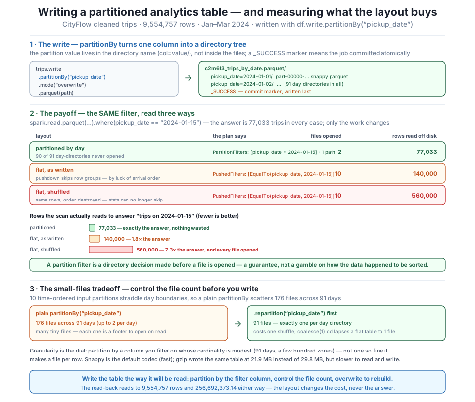
partitionBy("pickup_date") into 91 pickup_date=value directories with a _SUCCESS marker. Reading one day back, the same filter opens 1 directory of 91 — 2 files, 77,033 rows — via PartitionFilters, versus the flat table's all-10-files scan reading 140,000 rows (pushdown skipping by luck of arrival order) or 560,000 once shuffled. A plain partitionBy scatters 176 small files across 91 days; repartition("pickup_date") first collapses that to exactly 91, one per day. The table reads back to 9,554,757 rows and $256,692,373.14 — the layout changes the cost, never the answer.Clean up every table we wrote and close the session.
for p in [MODES, FLAT, PART, SHUF, PART1, FLAT1, GZIP]:
    if os.path.exists(p):
        shutil.rmtree(p)
if os.path.exists("spark-warehouse"):
    shutil.rmtree("spark-warehouse")
print("removed all c2m6l3_* artifacts")
spark.stop()
removed all c2m6l3_* artifacts_SUCCESS is a contract, not decoration
The empty _SUCCESS file is the cheapest reliability check in the whole pipeline. Spark writes it only after every part-* file has committed, so a downstream job that checks os.path.exists(path + "/_SUCCESS") before reading will never consume a half-written table left by a crash. Build that check into anything that reads a Spark output on a schedule — the marker is exactly what lets an orchestrator (Module 8’s subject) decide whether last night’s write is safe to use or needs a re-run.
Exercise 1 — Partition by borough instead of day, and count the files. The zone lookup (taxi_zone_lookup.csv) maps each PULocationID to a Borough (Manhattan, Queens, Brooklyn, Bronx, Staten Island, EWR, Unknown). Join it onto trips, then write the result partitionBy("Borough") into a c2m6l3_by_borough.parquet table. Count the partition directories and the total files, then read back just the Manhattan partition and confirm its row count. Compare the directory count to the 91 you got partitioning by day, and explain in a comment which partition key produces bigger, fewer files and why that matters for the small-files problem. Remove the table when done.
Hint
Borough has only about seven values, so you’ll get ~7 directories instead of 91 — far fewer, far larger files, no small-files risk at all, but much coarser pruning (a Manhattan filter still scans every Manhattan trip in the quarter). This is the cardinality dial in action: Borough is the coarse end, a per-second timestamp would be the catastrophic fine end, and pickup_date sits in the useful middle. Read one partition directly with spark.read.parquet(".../Borough=Manhattan"). Keep the c2m6l3_ prefix and shutil.rmtree at the end.
Exercise 2 — Prove the guarantee with a nested partition. Write trips partitioned by two columns, partitionBy("pickup_date", "PULocationID"), into c2m6l3_two_level.parquet (write a single month first — filter trips to January — so the directory count stays manageable). Inspect the on-disk layout: you should see pickup_date=.../PULocationID=.../ nested folders. Then filter on both columns for one day and one zone, call .explain(), and find both predicates in PartitionFilters with a Location of 1 paths. Use the scan_stats helper to confirm how few rows are read. Explain why nesting the partitions this way prunes even harder — and what it costs.
Hint
Two-level partitioning drills the pruning down to a single day-and-zone directory, so scan_stats will report a tiny row count read — but the cost is a combinatorial explosion of directories (days × zones), which is the small-files problem taken to an extreme. That’s exactly why you filtered to one month first: a full quarter × 260 zones would create thousands of tiny directories. The lesson generalizes: each partition level multiplies the directory count, so nest only when both columns are filtered together often and their combined cardinality stays sane.
Exercise 3 — Catch the append trap that Lesson 4 fixes. Write trips (filtered to a single day to keep it fast) to c2m6l3_append_trap.parquet with mode("overwrite") and record the row count. Now run the exact same write two more times with mode("append"), reading the count back after each. Watch the total grow. Then do it once more with mode("overwrite") and confirm the count snaps back to the true one-day figure. Write a comment explaining, in one sentence, why append is the wrong default for a re-runnable job and what property Lesson 4 will need to guarantee.
Hint
Each append adds the day’s rows again, so after two appends you’ll read three times the true count — a job that silently triples its output every time it’s retried. overwrite resets it to the correct number because it replaces rather than adds. The property you want is idempotency: running the job twice leaves the table identical to running it once. Keep the c2m6l3_ prefix and clean up; that idempotency guarantee, done efficiently for just the partitions a run touches, is exactly what the next lesson builds.
You turned CityFlow’s in-memory result into a written analytics table and measured what the write layout is worth. df.write.format("parquet").mode(...).save(path) lays a DataFrame down as a directory of part-* files plus a _SUCCESS marker that signals the job committed atomically, and mode decides the collision behaviour: overwrite replaced (5 rows), append added (5 → 10, the re-run trap), ignore skipped an existing path, and error raised AnalysisException. Written partitionBy("pickup_date"), the 9,554,757-row table became 91 pickup_date=value directories, and the payoff showed on read: the filter pickup_date == "2024-01-15" landed in PartitionFilters and opened 1 directory of 91 — 2 files, exactly 77,033 rows — while the identical filter on a flat table opened all 10 files and read 140,000 rows (pushdown skipping row groups only by luck of arrival order) or 560,000 once that order was shuffled away. Same 77,033-trip answer, an order-of-magnitude spread in work. The convenience cost a small-files problem — a plain partitionBy scattered 176 files across 91 days — which repartition("pickup_date") fixed to exactly 91, one per day, for the price of one shuffle. Snappy is the default codec (29.8 MB); gzip squeezed the same table to 21.9 MB at a read-time cost. And a full mode("overwrite") rebuild read back to 9,554,757 rows and $256,692,373.14 — the layout changed the cost, never the answer.
_SUCCESS — save(path) produces one part-* file per task, and the empty _SUCCESS marker appears only after all of them commit. Check for it before reading a scheduled output; its absence means a partial, untrustworthy write.mode is the collision policy — overwrite replaces, append adds (and silently double-counts a re-run), ignore is a no-op on an existing path, error refuses. For a rebuildable analytics table, overwrite is the safe default and append is the one to distrust.partitionBy writes the value into the directory name — one col=value/ folder per distinct value, and the column leaves the data files. A filter on a partition column becomes a PartitionFilters resolved against folder names before any file opens — here 1 directory of 91, 2 files, 77,033 rows.PartitionFilters prune the same way regardless of physical order, while PushedFilters skip only if the file’s row-group statistics happen to be tight (140,000 rows read when arrival order helped, 560,000 when shuffled). Partition by the column your queries filter on to convert luck into structure.repartition(col) before the write collapses them to one file per partition at the cost of a shuffle, coalesce(n) merges without one but only reduces. Pick a key whose cardinality is modest.The difference between a query and a job is that a job’s output is read by someone else, later, without you watching — and this lesson is where you take responsibility for that output. A teammate who writes the cleaned trips flat and reports “it’s Parquet, it’s fast” has told a half-truth: their one-day dashboard query reads 140,000 rows today because the source happened to arrive sorted, and 560,000 tomorrow when an upstream change scrambles the order, and nobody will know why the dashboard got slower. The engineer who writes partitionBy("pickup_date") has made that query read exactly the 77,033 rows it needs, forever, independent of how the data lands — and has done it not with a hand-tuned index but with one method call that bakes the access pattern into the directory structure. That is the shape of production data engineering: you don’t just compute the right answer, you lay it down so that everything downstream can get to its slice cheaply and predictably. The write is not the end of the pipeline; it is the interface the rest of the company reads through.
There is one loose thread in everything you just wrote, and it is the thread the next lesson pulls. Your nightly rebuild used mode("overwrite"), which replaced all 91 partitions even when a re-run only needed to fix one day — wasteful at best, and at worst the exact operation that overwrites data a run never meant to touch. And mode("append"), the mode that so conveniently added rows, quietly doubled the table every time the job ran twice. A production job gets retried: the scheduler fires it again after a timeout, an operator re-runs last night’s batch, the same file arrives twice. Lesson 4, Idempotent Jobs, makes the write safe under all of that. You’ll meet dynamic partition overwrite — the setting that lets overwrite replace only the partitions a run actually produced, leaving the other 90 days untouched — and prove, with the same 9,554,757-row table, that re-running one month changes nothing while a naive append doubles it. Writing the table correctly was this lesson; writing it so that running the job twice is indistinguishable from running it once is the next.
Keep DATATWEETS free. Help fund practical data, AI, and engineering lessons for learners worldwide.
