Lesson 5 - Guided Project: The Quarterly ETL

Welcome to the Quarterly ETL#

Every lesson in this module built one piece of a production job. Lesson 1 gave you the explicit schema — the contract that says what shape the data must have before you process a byte of it. Lesson 2 built the read-clean-transform body as functions that carry Course 1’s data-quality rules into Spark: the window filter, the reversals you must not delete, the zone join keyed on the id. Lesson 3 laid the result down as a partitioned Parquet table whose physical layout lets later reads skip whole files. Lesson 4 made the write idempotent with dynamic partition overwrite, so re-running a month replaces exactly that month’s partitions and never doubles the totals. Four disciplines, four lessons — and until now, four separate demos.

This project assembles them into one thing: a single quarterly_etl.py script, structured the way a real job is — typed functions, a run_etl() that wires them together, progress prints, a clean spark.stop() — that CityFlow could hand to a scheduler tonight. Then it proves the job is correct the only way that counts: it reads the written table back and cross-checks it against Course 1’s ground truth to the cent, and it runs the whole job a second time to show the totals do not move. That second run is the headline. A pipeline that produces the right answer once is a query; a pipeline that produces the same right answer every time you run it, without doubling or drifting, is a job you can trust to run unattended.

By the end of this project, you will be able to:

• Assemble a schema, a clean stage, a transform stage, and a partitioned write into one structured, reusable ETL script
• Preserve real data defects (the accounting reversals) instead of silently deleting them, and prove the dollar cost of getting that wrong
• Write a partitioned analytics table with a controlled file count, and verify it by reading it back rather than trusting the write
• Make the whole job idempotent, so re-running it replaces partitions instead of appending — and measure the doubling a naive append would cause
• Carry away a production-ETL checklist you can apply to any batch job

You’ll need pyspark with its Java runtime. Let’s build the job.

The Data and the One Session#

The data is New York City’s public-domain Yellow Taxi trip records — the same three months (January, February, March 2024) as the rest of the course, plus the zone lookup. Every runnable block below reads the local copies:

# gate: skip
# Fetch once; every block afterward reads the local cached copies by name.
import urllib.request
for m in ("01", "02", "03"):
    urllib.request.urlretrieve(
        f"https://d37ci6vzurychx.cloudfront.net/trip-data/yellow_tripdata_2024-{m}.parquet",
        f"yellow_tripdata_2024-{m}.parquet")
urllib.request.urlretrieve(
    "https://datatweets.com/datasets/nyc-taxi/taxi_zone_lookup.csv", "taxi_zone_lookup.csv")

One session for the whole project. We set one production-critical config up front: spark.sql.sources.partitionOverwriteMode = dynamic, the switch from Lesson 4 that makes an overwrite write replace only the partitions a run actually produces. We also declare the constants the job needs — the input files, the quarter’s window boundaries, and the output path — and the schema and zone-dimension helpers. This first block is the top of quarterly_etl.py:

import warnings; warnings.filterwarnings("ignore")
import datetime as dt, shutil, glob, os
from pyspark.sql import SparkSession, functions as F
from pyspark.sql.types import (StructType, StructField, IntegerType, LongType,
                               DoubleType, StringType, TimestampNTZType)

spark = (SparkSession.builder
         .appName("cityflow")
         .master("local[*]")
         .config("spark.ui.showConsoleProgress", "false")
         .getOrCreate())
spark.sparkContext.setLogLevel("ERROR")
spark.conf.set("spark.sql.sources.partitionOverwriteMode", "dynamic")

FILES = [f"yellow_tripdata_2024-{m}.parquet" for m in ("01", "02", "03")]
LO, HI = dt.datetime(2024, 1, 1), dt.datetime(2024, 4, 1)
OUT = "c2m6l5_zone_hour"

def log(msg):
    print(f"[etl] {msg}")

def taxi_schema():
    return StructType([
        StructField("VendorID", IntegerType()),
        StructField("tpep_pickup_datetime", TimestampNTZType()),
        StructField("tpep_dropoff_datetime", TimestampNTZType()),
        StructField("passenger_count", LongType()),
        StructField("trip_distance", DoubleType()),
        StructField("RatecodeID", LongType()),
        StructField("store_and_fwd_flag", StringType()),
        StructField("PULocationID", IntegerType()),
        StructField("DOLocationID", IntegerType()),
        StructField("payment_type", LongType()),
        StructField("fare_amount", DoubleType()),
        StructField("extra", DoubleType()),
        StructField("mta_tax", DoubleType()),
        StructField("tip_amount", DoubleType()),
        StructField("tolls_amount", DoubleType()),
        StructField("improvement_surcharge", DoubleType()),
        StructField("total_amount", DoubleType()),
        StructField("congestion_surcharge", DoubleType()),
        StructField("Airport_fee", DoubleType()),
    ])

def read_zone_dim():
    return (spark.read.option("header", True).csv("taxi_zone_lookup.csv")
            .select(F.col("LocationID").cast("int").alias("LocationID"), "Zone", "Borough"))

schema = taxi_schema()
zones = read_zone_dim()
print("schema fields     :", len(schema.fields))
print("zone dimension rows:", zones.count())

schema fields     : 19
zone dimension rows: 265

Nineteen typed fields and 265 zones — the contract and the dimension. Notice tpep_pickup_datetime is a TimestampNTZType: these records carry wall-clock timestamps with no zone, exactly as Lesson 1 established, and declaring that explicitly means Spark never has to guess it by scanning the file.

READ and CLEAN: Carry the Data’s Defects Forward Honestly#

The read is one line once the schema exists — spark.read.schema(schema).parquet(*files) pulls all three months without an inference pass. The clean stage is where the judgment lives, and it is the same judgment Course 1 earned the hard way. Three rules travel from that course into this Spark function:

1. Window filter, and quarantine what falls out. Keep only pickups in [2024-01-01, 2024-04-01). A handful of rows carry timestamps from outside the quarter — stray 2002 and 2023 dates, the classic dirty-timestamp defect. We don’t silently drop them; we quarantine them into a separate DataFrame so a later data-quality gate (Module 7) can inspect them.
2. Key on the id, never the name. Two different zones are both named “Corona”; the join must use PULocationID. Rows with a null PULocationID can’t be keyed, so they go to quarantine too.
3. Preserve the reversals. Some trips have a negative total_amount — accounting reversals, refunds, voided fares. The naive instinct is to “clean” them away as garbage. That instinct is a bug: those negatives are real money leaving the ledger, and deleting them inflates revenue. We keep them, and we flag suspicious trip_distance values with a column rather than dropping those rows either.

def read_trips(files, schema):
    return spark.read.schema(schema).parquet(*files)

def clean(raw):
    in_window = ((F.col("tpep_pickup_datetime") >= F.lit(LO)) &
                 (F.col("tpep_pickup_datetime") < F.lit(HI)))
    keyed = in_window & F.col("PULocationID").isNotNull()
    kept = raw.filter(keyed).withColumn(
        "distance_flag",
        F.when((F.col("trip_distance") <= 0) | (F.col("trip_distance") > 200), F.lit("suspect"))
         .otherwise(F.lit("ok")))
    quarantine = raw.filter(~keyed)
    return kept, quarantine

raw = read_trips(FILES, schema)
print("raw rows      :", f"{raw.count():,}")
kept, quarantine = clean(raw)
print("kept          :", f"{kept.count():,}")
print("quarantined   :", quarantine.count())

reversals = kept.filter(F.col("total_amount") < 0)
rev_sum = reversals.agg(F.round(F.sum("total_amount"), 2)).collect()[0][0]
full = kept.agg(F.round(F.sum("total_amount"), 2)).collect()[0][0]
dropped = kept.filter(F.col("total_amount") >= 0).agg(F.round(F.sum("total_amount"), 2)).collect()[0][0]
print("reversals kept:", f"{reversals.count():,}", "summing to", rev_sum)
print("phantom revenue if we dropped them:", round(dropped - full, 2))
kept.groupBy("distance_flag").count().orderBy("distance_flag").show()

raw rows      : 9,554,778
kept          : 9,554,757
quarantined   : 21
reversals kept: 115,894 summing to -2986808.76
phantom revenue if we dropped them: 2986808.76
+-------------+-------+
|distance_flag|  count|
+-------------+-------+
|           ok|9338823|
|      suspect| 215934|
+-------------+-------+

Read that middle line carefully, because it is the reason this stage is a function with a decision and not a one-liner. The quarter has 9,554,778 raw rows; the window filter keeps 9,554,757 and quarantines exactly 21 — matching Course 1 to the row. And there are 115,894 reversals in what we kept, summing to −$2,986,808.76. If a careless engineer had “cleaned out” the negative totals, revenue would have jumped by $2,986,808.76 of money that was never earned — nearly three million dollars of phantom revenue from a single well-intentioned filter. The distance_flag column marks 215,934 trips with a zero or absurd distance as suspect without deleting them; the row count is preserved so nothing silently vanishes. This is what “clean” means in production: not “throw away what looks odd,” but “keep everything real and label what’s questionable.”

TRANSFORM: The Zone-Hour Report#

The transform is the aggregation the whole course keeps returning to. Derive the hour bucket with date_trunc (a native expression — no UDF, so no JVM-to-Python round trip), join the tiny zone dimension with an explicit broadcast so nine million trips never shuffle to meet 265 rows, and group by zone and hour to count trips and sum revenue. We also derive a pickup_date column here — that will be the partition key when we write.

def transform(clean_df, zones):
    hourly = clean_df.withColumn("pickup_hour", F.date_trunc("hour", "tpep_pickup_datetime"))
    joined = hourly.join(F.broadcast(zones), hourly.PULocationID == zones.LocationID, "inner")
    return (joined.groupBy("PULocationID", "Zone", "pickup_hour")
            .agg(F.count(F.lit(1)).alias("trips"),
                 F.round(F.sum("total_amount"), 2).alias("revenue"))
            .withColumn("pickup_date", F.to_date("pickup_hour")))

report = transform(kept, zones)
b = report.count()
agg = report.agg(F.sum("trips").alias("trips"), F.round(F.sum("revenue"), 2).alias("revenue")).collect()[0]
print("zone-hour buckets:", f"{b:,}")
print("trips            :", f"{agg['trips']:,}")
print("revenue          :", f"${agg['revenue']:,.2f}")

zone-hour buckets: 240,917
trips            : 9,554,757
revenue          : $256,692,373.14

240,917 zone-hour buckets, 9,554,757 trips, $256,692,373.14 in revenue — the numbers this course has verified against a completely different engine. The trips total equals the kept-row count exactly, which is the arithmetic proof that the broadcast join dropped nothing: every kept trip found its zone. The report is in memory; now it has to become a table on disk that other systems can read.

WRITE: A Partitioned Analytics Table with a Controlled File Count#

The write stage does two production things at once. It partitions by pickup_date, so the physical layout on disk is a directory per day — a later query that wants one day reads one directory instead of scanning the whole table, the clustering win from Lesson 3. And it controls the file count: a naive partitioned write can scatter each partition across every task, producing a swarm of tiny files that later reads pay for. Calling repartition("pickup_date") before the write gathers each date’s rows onto one task first, so each partition lands as a single file.

def write_table(report, path):
    (report.repartition("pickup_date").write
     .mode("overwrite").partitionBy("pickup_date").parquet(path))

write_table(report, OUT)
parts = glob.glob(OUT + "/pickup_date=*")
files = glob.glob(OUT + "/pickup_date=*/*.parquet")
print("partitions written:", len(parts))
print("data files        :", len(files))

partitions written: 91
data files        : 91

91 partitions, 91 files — one clean file per day. Ninety-one, not ninety, because the first quarter of 2024 spans 31 + 29 + 31 days: February 2024 is a leap month. The mode("overwrite") combined with the dynamic config we set at the top means this write replaces partitions rather than blowing the whole table away — the property we’re about to lean on for idempotency.

VERIFY: Read the Table Back and Cross-Check#

Here is the discipline that separates a job you trust from one you hope about: verify by reading the written table back, not by trusting the DataFrame you just wrote. A write can succeed and still produce the wrong bytes — a partition column swallowed, a rounding drift, a silent type coercion. So we re-open the table from disk as if we were a downstream consumer, and cross-check it against Course 1’s ground truth to the cent.

def verify(path):
    back = spark.read.parquet(path)
    agg = back.agg(F.sum("trips").alias("trips"),
                   F.round(F.sum("revenue"), 2).alias("revenue")).collect()[0]
    return back, {"buckets": back.count(), "trips": agg["trips"], "revenue": agg["revenue"]}

back, m = verify(OUT)
print("read-back buckets:", f"{m['buckets']:,}")
print("read-back trips  :", f"{m['trips']:,}")
print("read-back revenue:", f"${m['revenue']:,.2f}")
print("\nbusiest pickup zones over the quarter:")
podium = (back.groupBy("PULocationID", "Zone").agg(F.sum("trips").alias("trips"))
          .orderBy(F.desc("trips")).limit(5).collect())
for r in podium:
    print(f"  {r['PULocationID']:>3}  {r['Zone']:<24}{r['trips']:>9,}")

read-back buckets: 240,917
read-back trips  : 9,554,757
read-back revenue: $256,692,373.14

busiest pickup zones over the quarter:
  161  Midtown Center            453,825
  237  Upper East Side South     439,138
  132  JFK Airport               429,745
  236  Upper East Side North     416,508
  162  Midtown East              336,460

The table on disk reads back to 240,917 buckets, 9,554,757 trips, and $256,692,373.14 — identical to what we computed in memory, and identical to Course 1’s capstone. The busiest-zone podium matches to the trip: Midtown Center on top at 453,825, then Upper East Side South, JFK, Upper East Side North, and Midtown East. The pickup_date partition column survived the round trip, the revenue rounding held, and every zone found its name. The write is trustworthy because we checked it, not because it returned without an error.

The Headline: Run the Whole Job Twice#

Now the proof this whole module has been building toward. A production ETL runs on a schedule, and schedules mean re-runs: a job retried after a failure, a day reprocessed because the source published a correction, a backfill that overlaps data already written. If a second run adds to the first instead of replacing it, every total silently doubles and the analytics downstream are wrong in a way no error message announces. The job must be idempotent: running it again must leave the output exactly as it was.

We assemble the pieces into a single run_etl() — the reusable job — and call it twice against the same output path. Because the write uses overwrite under the dynamic partition-overwrite mode, the second run replaces each of the 91 partitions with freshly computed, identical data. Then, to make the stakes concrete, we do the thing you must not do — one append — and measure the damage.

def run_etl():
    raw = read_trips(FILES, schema)
    kept_, _ = clean(raw)
    rep = transform(kept_, zones)
    write_table(rep, OUT)
    _, metrics = verify(OUT)
    return metrics

log("run A: full read -> clean -> transform -> write -> verify")
a = run_etl()
log("run B: exactly the same job again")
b2 = run_etl()
print("run A:", a)
print("run B:", b2)
print("idempotent (identical):", a == b2)

kept2, _ = clean(read_trips(FILES, schema))
transform(kept2, zones).write.mode("append").partitionBy("pickup_date").parquet(OUT)
_, appended = verify(OUT)
print("after one naive append:", appended)

shutil.rmtree(OUT)
if os.path.isdir("spark-warehouse"): shutil.rmtree("spark-warehouse")
spark.stop()

[etl] run A: full read -> clean -> transform -> write -> verify
[etl] run B: exactly the same job again
run A: {'buckets': 240917, 'trips': 9554757, 'revenue': 256692373.14}
run B: {'buckets': 240917, 'trips': 9554757, 'revenue': 256692373.14}
idempotent (identical): True
after one naive append: {'buckets': 481834, 'trips': 19109514, 'revenue': 513384746.28}

There it is. Run A and run B are byte-for-byte identical — 240,917 buckets, 9,554,757 trips, $256,692,373.14, twice, with idempotent == True. The job can run tonight, fail, retry, and run again, and the table it leaves behind is the same table every time. And the contrast is stark: a single append — the one wrong verb — doubled everything to 481,834 buckets, 19,109,514 trips, and $513,384,746.28. That doubling is the exact bug dynamic partition overwrite exists to prevent, and it’s the difference between a job you schedule and forget and a job you have to babysit and clean up after.

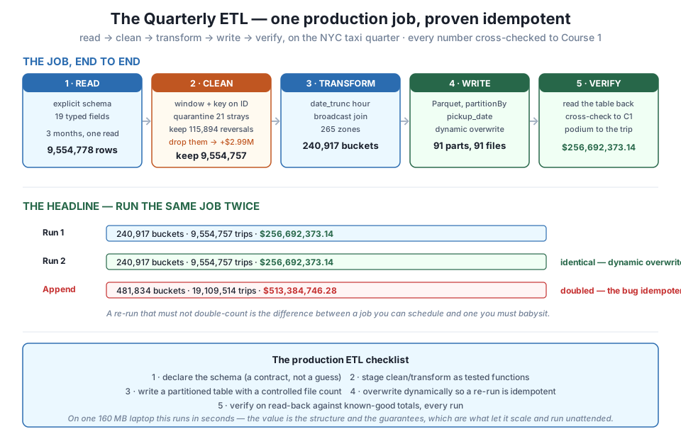
A word of honesty about scale. On this one 160 MB laptop, the entire ETL — read, clean, transform, write, verify, twice — finishes in a handful of seconds. Nothing here is impressive because it is fast. It is impressive because it is structured and guaranteed: an explicit schema contract, staged functions you can test in isolation, a partitioned output, and an idempotent write. Those are precisely the properties that stop mattering at 160 MB and start being the whole game at 160 terabytes on a real cluster, where a re-run that doubles the ledger is a production incident and a schema that drifts is a 3 a.m. page. You built the small version so the large version is the same code with more executors.

The Deliverable: quarterly_etl.py#

Everything above, assembled into the one file you keep. This is the same code you just ran, gathered into the shape a scheduler expects: importable functions, a main() that wires them and reports, and a __main__ guard. Nothing new runs here — it’s the takeaway artifact.

# gate: skip
# quarterly_etl.py — CityFlow's quarterly zone-hour ETL.
# Run: JAVA_HOME must point at a JDK 21; then `python quarterly_etl.py`.
import warnings; warnings.filterwarnings("ignore")
import datetime as dt
from pyspark.sql import SparkSession, functions as F
from pyspark.sql.types import (StructType, StructField, IntegerType, LongType,
                               DoubleType, StringType, TimestampNTZType)

FILES = [f"yellow_tripdata_2024-{m}.parquet" for m in ("01", "02", "03")]
LO, HI = dt.datetime(2024, 1, 1), dt.datetime(2024, 4, 1)
OUT = "zone_hour_report"

def log(msg):
    print(f"[etl] {msg}")

def build_session():
    spark = (SparkSession.builder.appName("cityflow-quarterly-etl")
             .master("local[*]")
             .config("spark.ui.showConsoleProgress", "false")
             .getOrCreate())
    spark.sparkContext.setLogLevel("ERROR")
    # replace only the partitions this run produces — the idempotency switch
    spark.conf.set("spark.sql.sources.partitionOverwriteMode", "dynamic")
    return spark

def taxi_schema():
    return StructType([
        StructField("VendorID", IntegerType()),
        StructField("tpep_pickup_datetime", TimestampNTZType()),
        StructField("tpep_dropoff_datetime", TimestampNTZType()),
        StructField("passenger_count", LongType()),
        StructField("trip_distance", DoubleType()),
        StructField("RatecodeID", LongType()),
        StructField("store_and_fwd_flag", StringType()),
        StructField("PULocationID", IntegerType()),
        StructField("DOLocationID", IntegerType()),
        StructField("payment_type", LongType()),
        StructField("fare_amount", DoubleType()),
        StructField("extra", DoubleType()),
        StructField("mta_tax", DoubleType()),
        StructField("tip_amount", DoubleType()),
        StructField("tolls_amount", DoubleType()),
        StructField("improvement_surcharge", DoubleType()),
        StructField("total_amount", DoubleType()),
        StructField("congestion_surcharge", DoubleType()),
        StructField("Airport_fee", DoubleType()),
    ])

def read_zone_dim(spark):
    return (spark.read.option("header", True).csv("taxi_zone_lookup.csv")
            .select(F.col("LocationID").cast("int").alias("LocationID"), "Zone", "Borough"))

def read_trips(spark, files):
    return spark.read.schema(taxi_schema()).parquet(*files)

def clean(raw):
    in_window = ((F.col("tpep_pickup_datetime") >= F.lit(LO)) &
                 (F.col("tpep_pickup_datetime") < F.lit(HI)))
    keyed = in_window & F.col("PULocationID").isNotNull()
    kept = raw.filter(keyed).withColumn(
        "distance_flag",
        F.when((F.col("trip_distance") <= 0) | (F.col("trip_distance") > 200), F.lit("suspect"))
         .otherwise(F.lit("ok")))            # flag, do not drop
    quarantine = raw.filter(~keyed)          # keep the strays for inspection, not the bin
    return kept, quarantine                  # reversals (negative totals) stay in `kept` on purpose

def transform(clean_df, zones):
    hourly = clean_df.withColumn("pickup_hour", F.date_trunc("hour", "tpep_pickup_datetime"))
    joined = hourly.join(F.broadcast(zones), hourly.PULocationID == zones.LocationID, "inner")
    return (joined.groupBy("PULocationID", "Zone", "pickup_hour")
            .agg(F.count(F.lit(1)).alias("trips"),
                 F.round(F.sum("total_amount"), 2).alias("revenue"))
            .withColumn("pickup_date", F.to_date("pickup_hour")))

def write_table(report, path):
    (report.repartition("pickup_date").write
     .mode("overwrite").partitionBy("pickup_date").parquet(path))

def verify(spark, path):
    back = spark.read.parquet(path)
    agg = back.agg(F.sum("trips").alias("trips"),
                   F.round(F.sum("revenue"), 2).alias("revenue")).collect()[0]
    return {"buckets": back.count(), "trips": agg["trips"], "revenue": agg["revenue"]}

def main():
    spark = build_session()
    try:
        zones = read_zone_dim(spark)
        log("reading three months under an explicit schema")
        raw = read_trips(spark, FILES)
        log("cleaning: window filter, key on LocationID, preserve reversals")
        kept, _quarantine = clean(raw)
        log("transforming to the zone-hour report")
        report = transform(kept, zones)
        log(f"writing partitioned table -> {OUT}")
        write_table(report, OUT)
        metrics = verify(spark, OUT)
        log(f"verified on read-back: {metrics}")
    finally:
        spark.stop()

if __name__ == "__main__":
    main()

And the production-ETL checklist the script embodies — the part you carry to the next job:

1. Declare the schema. It’s a contract, not a guess; inference costs a pass and fails silently when types drift.
2. Stage clean and transform as tested functions. Each is independently checkable, and each carries a data-quality decision on its face — preserve the reversals, quarantine the strays, key on the id.
3. Write a partitioned table with a controlled file count. Partition on the key downstream reads filter by; repartition before the write so you don’t strew tiny files.
4. Overwrite dynamically for idempotency. overwrite under partitionOverwriteMode=dynamic replaces the partitions a run produces and no others — a re-run is safe, a reprocess is surgical.
5. Verify on read-back, every run. Re-open the table from disk and cross-check against known-good totals. A write that returned without error is not a write you’ve checked.

Practice Exercises#

Exercise 1 — Prove idempotency partition by partition. The lesson showed the totals are identical across two runs. Prove it at the partition level: after run_etl(), capture spark.read.parquet(OUT).groupBy("pickup_date").agg(F.sum("trips"), F.sum("revenue")) as a small local list; run run_etl() again and capture the same; confirm the two per-date lists are equal. Then explain in one sentence why append would break this per-date check even though each individual date’s input never changed.

Exercise 2 — Reprocess one month, leave the others untouched. The real value of dynamic overwrite is surgical reprocessing. Write the full quarter, then call a version of the job on February only (["yellow_tripdata_2024-02.parquet"]) with the same OUT. Confirm that January’s and March’s partitions are byte-unchanged (same file count, same per-date totals) while February’s were rewritten. This is the incremental pattern Module 8 schedules.

Exercise 3 — Put a number on the reversal decision, per zone. The clean stage keeps 115,894 reversals worth −$2,986,808.76 across the quarter. Find where that correction lands: build two versions of the report — one from kept as-is, one from kept.filter(F.col("total_amount") >= 0) — join them on PULocationID/Zone, and report the five zones whose revenue would be most inflated by dropping the reversals. Which zone would look richest if you’d made the careless mistake?

Summary#

You assembled the entire module into one production job and proved it end to end. The script declares an explicit 19-field schema, reads three months (9,554,778 raw rows) in a single pass, and cleans them with the judgment Course 1 earned: a window filter keeping 9,554,757 trips and quarantining 21, a distance_flag marking 215,934 suspect distances without deleting them, and — the decision that matters most — preserving 115,894 reversals worth −$2,986,808.76, because dropping them would have invented $2,986,808.76 of revenue that was never earned. The transform derives the hour bucket with date_trunc, broadcast-joins the 265 zones, and produces the 240,917-bucket zone-hour report. The write lays it down as 91 partitioned Parquet files, one per day of the leap quarter, with a controlled file count. Reading the table back cross-checks to Course 1 to the cent — $256,692,373.14, with Midtown Center on top at 453,825 trips. And the headline: running the whole job a second time left every total identical, because dynamic partition overwrite replaces partitions instead of appending — while a single naive append doubled everything to 481,834 buckets and $513,384,746.28. On one laptop it runs in seconds; the point was never speed but structure and the idempotency guarantee.

Key Concepts#

• A schema is a contract you declare — production reads the taxi data with an explicit StructType, never inferring, so types can’t drift silently and no extra pass is spent guessing.
• Clean means label, not delete — the stray timestamps are quarantined, suspect distances are flagged, and the reversals are kept, because deleting negatives would have added $2,986,808.76 of phantom revenue.
• Partitioned writes with a controlled file count — partitionBy("pickup_date") after a repartition yields 91 tidy files that let later reads skip whole days instead of scanning the table.
• Idempotency is dynamic partition overwrite — overwrite under partitionOverwriteMode=dynamic replaces exactly the partitions a run produces, so a re-run leaves totals identical while append doubles them.
• Verify by reading back — re-open the written table and cross-check against known-good totals every run; a write that didn’t error is not a write you’ve confirmed.

Why This Matters#

The jobs CityFlow runs in production will never be watched. They fire at 2 a.m., read whatever the source dropped, and write a table the morning’s dashboards depend on — and sometimes they fail halfway, get retried, or reprocess a day the source corrected. The four disciplines in this script are exactly what make that safe: the schema catches a source that changed shape, the staged clean function preserves the real ledger instead of quietly inflating it, the partitioned write keeps reprocessing surgical, and the idempotent overwrite means a retry can never double the books. None of it depended on scale — the same code that ran this 160 MB quarter in seconds runs a hundred-terabyte quarter on a cluster with the same guarantees, which is the entire reason to build the job this way instead of typing the query and hoping. You now have a pipeline you could hand to a scheduler tonight and trust to be correct every night.

Continue Building Your Skills#

You’ve built a job that produces the right answer and produces it identically on every run — but it makes one dangerous assumption: that the data arriving each night is as clean as this quarter turned out to be. It won’t always be. A source can drop a file with the revenue column missing, a day where every timestamp is null, a February that suddenly has more rows than March — and this job, as written, would process the garbage without complaint and write a confidently wrong table. Module 7, Data Quality & Logging, adds the gates that make this pipeline fail loudly when its inputs are wrong: row-count and null-rate checks that halt the run before it writes, assertions that the totals land in a plausible range, and the structured logging that turns a silent 2 a.m. failure into an alert you can act on. The job you just built is trustworthy when the data is good; the next module is about making it trustworthy when the data is bad, which is the harder and more valuable half of production data engineering.