Title here
Summary here
Lesson 1 gave CityFlow a suite of executable validation rules — assertions the job evaluates against every batch, so a run can tell you whether the data it received was actually valid. That answers the first of Module 7’s three questions. This lesson answers the second, and it is the one most pipelines get wrong: what do you do with the rows that fail?
The reflex answer is filter(...) — remove them and carry on. It looks like hygiene and it passes code review, but it quietly destroys something you cannot get back. Once a row is filtered out it was never materialised: you cannot say which rows went, you cannot tell a reviewer why last night’s count moved by twenty-one, you cannot spot that the number of rejections tripled this week, and you certainly cannot re-ingest the rows after upstream fixes the bug that produced them. The alternative is the pattern this lesson builds: split the batch into good and quarantined instead of shrinking it, tag every quarantined row with the reason it was rejected, write both sides, and reconcile. The reconciliation is the backbone — a single line, checkable by anyone, that a silently-filtered pipeline can never produce: good + quarantined == input, measured on the real quarter as 9,554,757 + 21 = 9,554,778. Along the way we hold one line firmly: the 115,894 negative-total reversals stay in GOOD. They look strange, but looking strange is not a rule violation, and Module 6, Lesson 2 measured what removing them costs — $2,986,808.76 of revenue CityFlow never earned.
By the end of this lesson, you will be able to:
filter(...) destroys that a split preserves — and why “the counts moved” is unanswerable after a silent dropquarantine_reason using a single when-chain so every row carries at most one reason, then split it into good and quarantined framesreason and stamped with a run id and timestamp, then read it back and group by reason to see $98,383.85 held back across three rule classesYou’ll need pyspark with the JDK configured as in Module 1, Lesson 3, plus the three taxi-quarter Parquet files. Start the session and count the input.
Every claim in this lesson is measured against one number: how many rows this run actually received. Capture it once, up front, before anything is filtered, labelled, or split — because a reconciliation you compute after the cleaning has already run is not a check, it is a tautology:
import warnings
warnings.filterwarnings("ignore")

from pyspark.sql import SparkSession, functions as F

spark = (SparkSession.builder
         .appName("cityflow")
         .master("local[*]")
         .config("spark.ui.showConsoleProgress", "false")
         .getOrCreate())
spark.sparkContext.setLogLevel("ERROR")

QUARTER = ["yellow_tripdata_2024-01.parquet",
           "yellow_tripdata_2024-02.parquet",
           "yellow_tripdata_2024-03.parquet"]

raw = spark.read.parquet(*QUARTER)
INPUT_ROWS = raw.count()
print(f"input rows for this run: {INPUT_ROWS:,}")
input rows for this run: 9,554,7789,554,778 rows — Course 1’s verified quarter total, and from here on the only number the outputs have to add up to. Note the discipline in that variable: INPUT_ROWS is a Python int captured at read time, not a lazy expression re-evaluated later. It is the fixed point of the run, and everything downstream is measured against it.
Start with the version almost every first-draft pipeline ships. The quarter window is a legitimate rule — CityFlow’s report is about January through March 2024, so a pickup outside that range does not belong in it. The obvious implementation removes them:
in_window = ((F.col("tpep_pickup_datetime") >= "2024-01-01") &
             (F.col("tpep_pickup_datetime") <  "2024-04-01"))

survivors = raw.filter(in_window)
print(f"input     : {INPUT_ROWS:,}")
print(f"survivors : {survivors.count():,}")
print(f"difference: {INPUT_ROWS - survivors.count():,}")
print("what were those rows? -> the DataFrame cannot say; they were never materialised")
input : 9,554,778
survivors : 9,554,757
difference: 21
what were those rows? -> the DataFrame cannot say; they were never materialisedThe arithmetic is right and the answer is right, and that is exactly what makes this dangerous. 21 rows disappeared and survivors has no memory of them. Ask the four questions an on-call engineer actually asks at 8 a.m. and watch every one of them fail:
survivors. You could re-read the source and re-derive them — but only because this source is a static file you still have. A pipeline reading a stream, a truncated staging table, or a vendor drop that gets rotated after a week cannot go back.None of these are hypothetical. A feed that starts sending 3% bad rows instead of 0.0002% is the single most common way a pipeline goes quietly wrong, and a silent filter is precisely the mechanism that hides it — the job keeps succeeding, the row count drifts down, and the first person to notice is whoever reads the dashboard three weeks later. The fix is not to stop rejecting rows. It is to stop rejecting them silently.
The pattern has two moves, and keeping them separate is what makes it maintainable. First, label: add a quarantine_reason column, evaluated for every row, that names the rule the row broke or is NULL if it broke none. Second, split: partition the frame on that column. Labelling with a single when-chain gives you a property worth naming — because when short-circuits at the first matching branch, every row gets at most one reason, which is what makes counting by reason a clean partition of the batch rather than an overlapping tally:
out_of_window = ((F.col("tpep_pickup_datetime") <  "2024-01-01") |
                 (F.col("tpep_pickup_datetime") >= "2024-04-01"))

def label_quality(df):
    """Tag every row with the FIRST rule it violates, or NULL if it violates none."""
    return df.withColumn(
        "quarantine_reason",
        F.when(out_of_window, F.lit("out_of_window"))
         .otherwise(F.lit(None).cast("string")))

labelled = label_quality(raw)
labelled.groupBy("quarantine_reason").count().orderBy("quarantine_reason").show(truncate=False)
+-----------------+-------+
|quarantine_reason|count |
+-----------------+-------+
|NULL |9554757|
|out_of_window |21 |
+-----------------+-------+Note that out_of_window is written as the negation of the window predicate, not as ~in_window. Both work here, but stating a rule in the positive — “this row is out of window because its pickup is before the start or at-or-after the end” — is what you want in the code, because that sentence is the thing you are recording in the data. A reason column whose values are named after rules is a column a reviewer can read.
Now the split, which is deliberately trivial:
def split_batch(df):
    """One labelled frame in, two frames out: good and quarantined."""
    good = df.filter(F.col("quarantine_reason").isNull()).drop("quarantine_reason")
    quarantined = df.filter(F.col("quarantine_reason").isNotNull())
    return good, quarantined

good, quarantined = split_batch(labelled)

good_rows = good.count()
quarantined_rows = quarantined.count()

print(f"good        : {good_rows:,}")
print(f"quarantined : {quarantined_rows:,}")
print(f"sum         : {good_rows + quarantined_rows:,}")
print(f"input       : {INPUT_ROWS:,}")
print(f"reconciles  : {good_rows + quarantined_rows == INPUT_ROWS}")

assert good_rows + quarantined_rows == INPUT_ROWS, "rows vanished between input and outputs"
good : 9,554,757
quarantined : 21
sum : 9,554,778
input : 9,554,778
reconciles : TrueThere it is, and it deserves a name because the rest of the module leans on it. The reconciliation identity is the claim that the batch was partitioned, not shrunk:
Measured here as 9,554,757 + 21 = 9,554,778. It is one line, it takes a reviewer two seconds, and it is structurally impossible to produce after a silent filter — you would have no second number to add. Note it is written as an assert, not a print: a reconciliation that only gets logged is a reconciliation nobody reads. Made an assertion, it becomes a rule the job enforces on itself, and Lesson 4 will turn that assertion into a proper exit code.
The identity catches bugs no per-rule count can
It is easy to read good + quarantined == input as bookkeeping — of course a filter and its complement add up. That is true only while the two sides really are complements. The moment a pipeline grows a second cleaning stage, a dropDuplicates, a join that fans out or drops non-matches, or a rule accidentally written with and where or was meant, the sides stop being complements and the sum stops matching. That is the whole point: the identity does not verify your rules are correct, it verifies your pipeline is conservative — that no row left the building without being written down somewhere. Rule correctness is Lesson 1’s job; row conservation is this one’s.
Quarantined rows are only useful if somebody looks at them, and looking is now possible — they are a DataFrame, not a memory of a filter. Here is what the window rule actually caught in this quarter:
(quarantined
 .select("tpep_pickup_datetime", "tpep_dropoff_datetime",
         "trip_distance", "total_amount", "PULocationID", "quarantine_reason")
 .orderBy("tpep_pickup_datetime")
 .show(8, truncate=False))
+--------------------+---------------------+-------------+------------+------------+-----------------+
|tpep_pickup_datetime|tpep_dropoff_datetime|trip_distance|total_amount|PULocationID|quarantine_reason|
+--------------------+---------------------+-------------+------------+------------+-----------------+
|2002-12-31 22:17:10 |2002-12-31 22:42:24 |1.4 |18.0 |50 |out_of_window |
|2002-12-31 22:59:39 |2002-12-31 23:05:41 |0.63 |-10.5 |170 |out_of_window |
|2002-12-31 22:59:39 |2002-12-31 23:05:41 |0.63 |10.5 |170 |out_of_window |
|2002-12-31 23:08:30 |2003-01-01 14:58:35 |5.34 |25.15 |132 |out_of_window |
|2008-12-31 22:52:49 |2008-12-31 23:04:09 |1.62 |19.9 |141 |out_of_window |
|2009-01-01 00:02:13 |2009-01-01 00:48:28 |0.57 |17.16 |79 |out_of_window |
|2009-01-01 00:24:09 |2009-01-01 01:13:00 |10.88 |68.29 |138 |out_of_window |
|2009-01-01 23:30:39 |2009-01-02 00:01:39 |10.99 |50.0 |237 |out_of_window |
+--------------------+---------------------+-------------+------------+------------+-----------------+
only showing top 8 rowsThis table is the argument for the whole pattern, because it tells you things. The first row is the famous stray — a pickup stamped 2002-12-31 22:17:10, hiding in the March file, a meter whose clock was never set. The next two rows are more interesting still: an identical pickup time, an identical distance, and totals of −10.50 and +10.50 — a reversal pair, in quarantine, with the same broken 2002 clock. Rows four through eight cluster around 2002-12-31, 2008-12-31, and 2009-01-01, which is not random noise: those are default epochs a meter falls back to when its clock resets. The remaining rows (not shown here) sit on 2023-12-31 and 2024-04-01 — genuine boundary spill from trips that started minutes on the wrong side of the quarter.
That is a diagnosis, and it came from reading the rejects. A filter would have given you the number 21 and nothing else. Now consider what changes if next month’s file quarantines 40,000 rows all stamped 2009-01-01: you would know within a minute that a batch of meters reset, which vendor they belong to, and that the trips are real trips with a broken clock rather than junk — a repair, not a deletion. Bad rows are data about your pipeline.
Now the discipline that keeps quarantine honest. It is tempting, once you have a quarantine table, to send everything suspicious to it. Resist that, and the reversals are the case that proves why. Check what stayed in GOOD:
g = good.agg(F.count(F.lit(1)).alias("rows"),
             F.sum((F.col("total_amount") < 0).cast("int")).alias("reversals"),
             F.round(F.sum("total_amount"), 2).alias("revenue")).first()

print(f"good rows      : {g['rows']:,}")
print(f"reversals kept : {g['reversals']:,}")
print(f"good revenue   : ${g['revenue']:,.2f}")
good rows : 9,554,757
reversals kept : 115,894
good revenue : $256,692,373.14All 115,894 negative-total_amount rows are in GOOD, and the good table sums to $256,692,373.14 — Course 1’s verified quarterly revenue, to the cent. Those reversals are the single most quarantine-tempting thing in this dataset: negative money looks like corruption. But they are not rule violations. They are a charge billed and voided, deliberately left in the ledger as an offsetting pair so that SUM cancels them, and Module 6 measured that removing them inflates revenue by $2,986,808.76. Quarantining them would be exactly as wrong as filtering them — it would just be wrong in a folder you can inspect.
The test to apply before quarantining anything is: can I name the rule this row breaks? “Out of the reporting window” is a rule. “Dropoff before pickup” is a rule. “Negative total” is a hunch, and a wrong one. A quarantine table that fills with rows nobody can name a rule for is not a safety mechanism; it is a place where correct data goes to be forgotten, with the added insult that the numbers now look defensible because they came out of a “quality” process.
One rule makes a thin demonstration. Real ingests carry several, and the when-chain scales to them directly. Here is a stricter policy with three rules — and this is a genuine design decision with a measurable cost, so we make it explicitly rather than by default:
def label_quality_strict(df):
    return df.withColumn(
        "quarantine_reason",
        F.when(out_of_window, F.lit("out_of_window"))
         .when(F.col("trip_distance") > 1000, F.lit("suspect_distance"))
         .when(F.col("tpep_dropoff_datetime") <= F.col("tpep_pickup_datetime"),
               F.lit("impossible_duration"))
         .otherwise(F.lit(None).cast("string")))

strict = label_quality_strict(raw)
good_strict, quarantined_strict = split_batch(strict)

quarantined_strict.groupBy("quarantine_reason").count().orderBy("quarantine_reason").show(truncate=False)

gs = good_strict.agg(F.count(F.lit(1)).alias("rows"),
                     F.sum((F.col("total_amount") < 0).cast("int")).alias("reversals"),
                     F.round(F.sum("total_amount"), 2).alias("revenue")).first()
qs_rows = quarantined_strict.count()

print(f"good (strict)      : {gs['rows']:,}")
print(f"quarantined (strict): {qs_rows:,}")
print(f"sum                : {gs['rows'] + qs_rows:,}  == input {INPUT_ROWS:,} -> {gs['rows'] + qs_rows == INPUT_ROWS}")
print(f"reversals kept     : {gs['reversals']:,}")
print(f"revenue (strict)   : ${gs['revenue']:,.2f}")
print(f"revenue withheld   : ${g['revenue'] - gs['revenue']:,.2f}")
+-------------------+-----+
|quarantine_reason |count|
+-------------------+-----+
|impossible_duration|2801 |
|out_of_window |21 |
|suspect_distance |158 |
+-------------------+-----+
good (strict) : 9,551,798
quarantined (strict): 2,980
sum : 9,554,778 == input 9,554,778 -> True
reversals kept : 115,884
revenue (strict) : $256,593,989.29
revenue withheld : $98,383.85Read the tradeoff honestly, because it is the real content of this section. The stricter policy quarantines 2,980 rows instead of 21: 21 out of window, 158 with a trip_distance over 1,000 miles (Module 6’s 312,722.3-mile odometer is the worst of them), and 2,801 whose dropoff is at or before their pickup. Every one of those is a nameable rule violation, so the quarantine is legitimate. But it costs — the good table now sums to $256,593,989.29, holding back $98,383.85 of revenue and no longer matching Course 1’s published total. That is not a bug; it is the point. Stricter validation is not free, and the price is stated in dollars rather than felt as a vague loss.
Two things did not change. The reconciliation identity still holds exactly — 9,551,798 + 2,980 = 9,554,778 — which is the property worth internalising: change the rules and both sides move together, but the sum never does. And the reversals still stay in GOOD: 115,884 of them, ten fewer than before only because ten reversal rows happen to also violate one of the new rules (two of them are the 2002 pair you saw above). Not one reversal was quarantined for being negative.
Which policy should CityFlow ship? For the published quarterly revenue report, the one-rule policy, because a zero-duration trip still represents money that changed hands and withholding it makes the report disagree with the vendor’s ledger. For a trip-duration study, the strict policy, because a dropoff before its pickup would poison every duration statistic. The rules belong to the question you are answering — and because both policies write their rejects rather than dropping them, you can change your mind later without re-reading the source.
A split that lives only in memory is not yet a quarantine pattern. Both frames get written, and the quarantine table gets two pieces of metadata that turn it from a dump into something queryable: a run id identifying which execution rejected the row, and a timestamp. Partitioning by quarantine_reason means a reviewer asking “show me the suspect distances” reads one directory instead of scanning the table:
import datetime as dt

RUN_ID = "2024Q1-" + dt.datetime.now().strftime("%Y%m%dT%H%M%S")
GOOD_PATH = "c2m7l2_trips_good.parquet"
QUARANTINE_PATH = "c2m7l2_trips_quarantine.parquet"

stamped = (quarantined_strict
           .withColumn("run_id", F.lit(RUN_ID))
           .withColumn("quarantined_at", F.current_timestamp()))

good_strict.write.mode("overwrite").parquet(GOOD_PATH)
(stamped.write
        .mode("overwrite")
        .partitionBy("quarantine_reason")
        .parquet(QUARANTINE_PATH))

print("run id:", RUN_ID)
import os
for d in sorted(os.listdir(QUARANTINE_PATH)):
    print(" ", d)
run id: 2024Q1-20260718T141542
._SUCCESS.crc
_SUCCESS
quarantine_reason=impossible_duration
quarantine_reason=out_of_window
quarantine_reason=suspect_distanceYour run id will differ — it encodes the wall-clock time of the run, which is the whole idea. The directory listing is the payoff of partitionBy: the reason is now part of the path, exactly the layout Module 6, Lesson 3 measured for the analytics table, applied to rejects. A query filtering on quarantine_reason prunes to one directory before opening a file. Both writes use mode("overwrite") so a re-run replaces its own output rather than doubling it — the idempotence discipline from Module 6, Lesson 4, which matters more for quarantine than for the good table, since a quarantine table that accumulates duplicates on every retry will have you chasing a phantom rejection spike.
Why the run id has to be in the row, not the folder name
It is tempting to encode the run in the output path (quarantine/2024Q1-.../) and leave the rows clean. Stamp the row instead. A quarantine table is read by union across many runs — “how have rejections trended since March?” — and a run id inside the row survives that union, while a path-encoded one is lost the moment two runs are read together. The same argument applies to quarantined_at. These two columns cost a few bytes per rejected row and are what make the table answer questions about the pipeline rather than only about the data. Lesson 3 uses the same run id to tie a structured log line to the rows it describes.
The identity we asserted earlier was computed on lazy DataFrames. The one that matters to an auditor is computed on what actually landed — because that is the version that catches a failed write, a partial commit, or a path someone overwrote by hand:
back_good = spark.read.parquet(GOOD_PATH)
back_quarantine = spark.read.parquet(QUARANTINE_PATH)

wrote_good = back_good.count()
wrote_quarantine = back_quarantine.count()
print(f"good on disk       : {wrote_good:,}")
print(f"quarantine on disk : {wrote_quarantine:,}")
print(f"total on disk      : {wrote_good + wrote_quarantine:,}  (input {INPUT_ROWS:,})")
print(f"RECONCILED         : {wrote_good + wrote_quarantine == INPUT_ROWS}")

(back_quarantine.groupBy("quarantine_reason", "run_id")
                .agg(F.count(F.lit(1)).alias("rows"),
                     F.round(F.sum("total_amount"), 2).alias("withheld_revenue"))
                .orderBy("quarantine_reason")
                .show(truncate=False))
good on disk : 9,551,798
quarantine on disk : 2,980
total on disk : 9,554,778 (input 9,554,778)
RECONCILED : True
+-------------------+----------------------+----+----------------+
|quarantine_reason |run_id |rows|withheld_revenue|
+-------------------+----------------------+----+----------------+
|impossible_duration|2024Q1-20260718T141542|2801|93185.92 |
|out_of_window |2024Q1-20260718T141542|21 |540.39 |
|suspect_distance |2024Q1-20260718T141542|158 |5197.93 |
+-------------------+----------------------+----+----------------+9,551,798 + 2,980 = 9,554,778, reconciled against bytes on disk rather than against a plan. And the grouped table is the artefact this whole lesson exists to produce: a per-reason breakdown, attributable to a run, with the withheld revenue attached — $93,185.92 in zero-or-negative-duration trips, $540.39 in out-of-window strays, $5,197.93 in broken odometers, summing to the $98,383.85 the strict policy holds back. Note that quarantine_reason comes back as a real column even though it exists only as a directory name on disk: Spark recovers partition columns from the path when it reads the table, so partitioning cost nothing in queryability.
That table is what you put in front of a reviewer, and what a monitoring job diffs week over week. If impossible_duration jumps from 2,801 to 300,000 next month, nobody has to discover it — the number is a column in a table that already exists.
Quarantine is a stage, not a graveyard. Rows land there, a human or a rule reviews them, and each class ends up either repaired-and-re-ingested or accepted-as-rejected. Start with the review — look at the worst offenders in one class:
(back_quarantine
 .filter(F.col("quarantine_reason") == "suspect_distance")
 .select("tpep_pickup_datetime", "trip_distance", "total_amount", "PULocationID")
 .orderBy(F.col("trip_distance").desc())
 .show(5, truncate=False))
+--------------------+-------------+------------+------------+
|tpep_pickup_datetime|trip_distance|total_amount|PULocationID|
+--------------------+-------------+------------+------------+
|2024-01-30 06:37:00 |312722.3 |22.15 |151 |
|2024-02-07 06:56:00 |222478.29 |18.89 |263 |
|2024-03-07 07:41:00 |176836.3 |32.74 |263 |
|2024-03-29 10:43:00 |176744.79 |114.68 |48 |
|2024-03-22 07:35:00 |176329.23 |34.51 |262 |
+--------------------+-------------+------------+------------+
only showing top 5 rowsNow read that, because it settles the design question. The distances are impossible — 312,722 miles is more than the distance to the Moon — but look at total_amount: $22.15, $18.89, $32.74. Those are ordinary Manhattan fares. These are not fake trips. They are real trips whose distance field is broken, most likely a meter reporting in the wrong unit or a sensor fault. The correct disposition is therefore not “reject the row” but “reject the field”: null the distance, keep the trip, and let the revenue count. That is a repair, and re-ingesting it is exactly what a quarantine table exists to make possible:
repaired = (back_quarantine
            .filter(F.col("quarantine_reason") == "suspect_distance")
            .withColumn("trip_distance", F.lit(None).cast("double"))
            .select(back_good.columns))

reingested = back_good.unionByName(repaired)
r = reingested.agg(F.count(F.lit(1)).alias("rows"),
                   F.round(F.sum("total_amount"), 2).alias("revenue")).first()
still_out = wrote_quarantine - repaired.count()

print(f"good after re-ingest : {r['rows']:,}")
print(f"still quarantined    : {still_out:,}")
print(f"sum                  : {r['rows'] + still_out:,}  (input {INPUT_ROWS:,})")
print(f"revenue recovered    : ${r['revenue'] - gs['revenue']:,.2f}")
print(f"revenue now          : ${r['revenue']:,.2f}")
good after re-ingest : 9,551,956
still quarantined : 2,822
sum : 9,554,778 (input 9,554,778)
revenue recovered : $5,197.93
revenue now : $256,599,187.22158 rows came back — good rises to 9,551,956, quarantine falls to 2,822, $5,197.93 of real revenue is recovered, and 9,551,956 + 2,822 = 9,554,778 still holds. That last part is the discipline: re-ingestion moves rows between the two sides, never into or out of the pipeline, so the identity survives the correction. Had you filtered instead of quarantined, recovering that $5,197.93 would have required re-reading and re-cleaning the entire source — assuming it still existed.
The other two classes get the opposite decision, and deciding is the job. The 21 out_of_window rows are accepted as rejected: they are genuinely not part of this quarter, and the right follow-up is a note to the vendor about meter clocks, not a re-ingest. The 2,801 impossible_duration rows deserve a real conversation — $93,185.92 is not a rounding error, and if those turn out to be legitimate minimum-charge waits recorded with a coarse clock, the rule is what needs fixing, not the rows. Either way the row count in the report changes only through a decision somebody made and can point at.
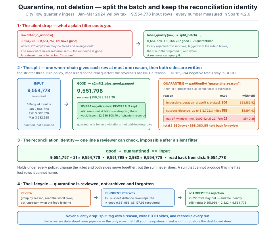
filter takes 9,554,778 to 9,554,757 and destroys the 21 rejected rows; label_quality plus split_batch keeps them, tagged. Under the stricter policy the batch splits into 9,551,798 good (all 115,884 reversals retained, $256,593,989.29) and 2,980 quarantined across impossible_duration 2,801, suspect_distance 158, and out_of_window 21 — $98,383.85 held back. The identity holds every way it is measured: 9,554,757 + 21, 9,551,798 + 2,980, and after re-ingesting 158 repaired rows 9,551,956 + 2,822 — always 9,554,778.The quarter’s good table is 9.5 million rows on disk and this lesson’s copy has served its purpose. Remove both tables and stop the session:
import shutil

for path in (GOOD_PATH, QUARANTINE_PATH, "spark-warehouse"):
    shutil.rmtree(path, ignore_errors=True)

spark.stop()
print("temporary tables removed; session stopped")
temporary tables removed; session stoppedExercise 1 — Add a referential rule and re-reconcile. Lesson 1’s referential check found 0 orphaned PULocationID values against the 265-row zone dimension — but the junk zone codes 264 and 265 are referentially valid and analytically meaningless. Add a fourth branch to label_quality_strict that tags rows whose PULocationID is 264 or 265 with the reason unknown_zone, re-run the split, and print the per-reason counts. Then assert the reconciliation identity again and report the new good count, the new withheld revenue, and how many rows the new rule stole from each of the existing reason classes.
Hint
Put the new branch last in the when-chain and the existing three counts will not move at all — a row already tagged out_of_window short-circuits before reaching it. Put it first and some rows will migrate between classes, and the totals will differ. Run it both ways: the difference between the two per-reason tables is a concrete demonstration that a when-chain expresses rule precedence, and that the order is a design decision you should make deliberately rather than by accident of typing.
Exercise 2 — Make the reconciliation a reusable function. Write reconcile(input_rows, good_df, quarantined_df) that counts both sides, prints a three-line report (good, quarantined, sum vs input), and raises a ValueError naming the shortfall if they disagree. Then deliberately break it: insert a .dropDuplicates() into the good branch of split_batch before reconciling, and watch the function catch the rows that silently vanished. Report how many duplicate rows the quarter actually contains.
Hint
dropDuplicates() across all 19 columns is a full shuffle on a 9.5 million-row frame, so expect it to be the slowest thing in the lesson — run it once and reuse the count. The failure message is the part worth designing: f"lost {input_rows - good - quarantined:,} rows" tells an on-call engineer more than assert alone ever will, and it is exactly the shape Lesson 4 turns into a nonzero exit code.
Exercise 3 — Simulate two runs and trend the rejections. The run id exists so quarantine can be read across runs. Write the quarantine table twice with mode("append") and two different run ids — the second time from a deliberately degraded input (for example, only the March file, or the quarter with the window rule tightened to February only) — then read the combined table and produce a groupBy("run_id", "quarantine_reason") report showing how each reason class moved between runs. Which class changed the most, and would a threshold alarm on that column have fired?
Hint
mode("append") is correct here and wrong in production for the same path within one run — appending on a retry double-counts, which is why the lesson used overwrite. A real quarantine table gets the run into the layout, for example partitionBy("run_id", "quarantine_reason"), so each run overwrites only its own partition. Try that variant and look at the resulting directory tree: it is the shape that makes both “this run’s rejects” and “this reason over time” cheap to query.
The reflex response to a bad row — filter(...) — is the one response that cannot be audited: it removes 21 rows from CityFlow’s 9,554,778-row quarter and leaves no record of which rows, which rule, or whether 21 is normal. This lesson replaced the drop with a split. label_quality tags every row with the first rule it violates using a short-circuiting when-chain, so each row carries at most one quarantine_reason; split_batch partitions the frame into good and quarantined; and both sides are written. The window rule alone yields 9,554,757 good and 21 quarantined — including the meter stamped 2002-12-31 22:17:10 in the March file, and a reversal pair sharing the same broken clock — with all 115,894 negative-total reversals retained in GOOD and the good table summing to Course 1’s $256,692,373.14 to the cent, because quarantine is for rows that break a nameable rule, not rows that look odd. A stricter three-rule policy quarantines 2,980 rows (out_of_window 21 / $540.39, suspect_distance 158 / $5,197.93, impossible_duration 2,801 / $93,185.92), leaving 9,551,798 good at $256,593,989.29 and holding $98,383.85 back — a real cost, stated in dollars rather than assumed away. Through all of it runs the reconciliation identity: good + quarantined == input, asserted rather than printed, and measured at 9,554,757 + 21, 9,551,798 + 2,980, on disk after the write, and again at 9,551,956 + 2,822 after 158 repaired odometer rows were re-ingested for $5,197.93 — 9,554,778 every single time. The quarantine table itself is written partitionBy("quarantine_reason") and stamped with a run id and timestamp, so a reviewer groups by reason in one query, a monitor diffs the counts week over week, and a fix upstream can bring rows back.
filter destroys the rejected rows, so the four questions an on-call engineer asks (which rows, why, is this normal, can we recover them) all become unanswerable; a split answers all four because the rejects are still a table.when-chain assigns each row at most one quarantine_reason (it short-circuits, so branch order encodes rule precedence), and split_batch turns that column into two frames; the labelling is the rule logic, the split is trivial.The difference between a pipeline that runs and a pipeline you can trust is almost never the correctness of its arithmetic — it is whether the job can account for itself afterwards. Rows will always be rejected; feeds drift, meters break, clocks reset. What separates a mature ingest from a fragile one is that the mature one can hand you a table of exactly what it rejected, why, and when, and prove in one line that nothing else went missing. That capability is what turns a data quality process from an assertion of good intentions into evidence. It is also what makes recovery possible: when the vendor fixes the meters next month, CityFlow re-ingests 158 rows and recovers $5,197.93 in an afternoon instead of re-processing a quarter. And it is what makes drift visible — a rejection count that has been a column in a table since day one is a number you can alarm on, while a rejection count that was never written down is a discovery someone makes weeks too late. Every downstream guarantee this module builds depends on this one: you cannot log what a run did, or fail loudly when a run went wrong, if the run has already thrown away the evidence.
You can now split a batch, name every rejection, write both sides, and prove that nothing vanished. What you cannot yet do is answer the question somebody will ask at nine in the morning: what did last night’s run actually do? The counts you printed to the console are gone the moment the terminal scrolls, and a print is not something a machine can read. Lesson 3, Structured Logging, gives the job a memory: Python’s logging configured properly for a Spark driver, and — more importantly — structured output, key-value or JSON lines that are greppable and parseable rather than prose nobody can query. You’ll log the numbers this lesson produced as a machine-readable run summary tied to the same run id you stamped into the quarantine table (read 9,554,778 in, 9,554,757 good, 21 quarantined, 240,917 buckets out, $256,692,373.14 total), measure the honest cost of all that counting — every count() is an action that re-triggers work, the caching tradeoff from Module 5 — and label your stages with setJobDescription so the Spark UI shows what a stage means instead of a line number. The split gave you the facts; next you make the run remember them.
Keep DATATWEETS free. Help fund practical data, AI, and engineering lessons for learners worldwide.
