Title here
Summary here
Lesson 1 gave the pipeline a set of executable validation rules, and Lesson 2 gave it a place to put the rows that fail them — a quarantine path with reasons attached, so that 21 stray timestamps get inspected rather than deleted. Both lessons assumed somebody was sitting at the terminal watching the output scroll by. Tonight nobody will be. The job fires at 2 a.m., reads whatever the source dropped, writes a table the morning’s dashboards depend on, and finishes before anyone is awake. When you open your laptop at nine and someone asks “did last night’s run go okay?”, the only evidence you have is whatever the job wrote down about itself.
That is what this lesson builds: a run log that answers “what did last night’s run actually do?” without re-running anything. We configure Python’s logging module properly for a Spark job, then make the crucial move from prose to structure — stage=clean rows_in=9554778 rows_out=9554757 quarantined=21 instead of "finished cleaning, looks fine" — because the first is greppable and machine-parseable and the second is a feeling. We close the run with a single JSON line and parse it straight back to prove it. And then we do the thing this course insists on: we measure what the logging costs. Every count in those lines is a Spark action, and asking for them naively re-ran the pipeline over and over. The measured penalty on this quarter was 1.51x for byte-identical log output. Observability is not free, and knowing its price is what lets you spend it deliberately.
By the end of this lesson, you will be able to:
logging module for a Spark job with a level, a timestamped format carrying a run id, and both console and file handlerskey=value stage records instead of prose prints, and explain why one is operable and the other is notjson.loads to compare runs night over nightYou’ll need pyspark with its Java runtime, plus logging, json, and uuid from the standard library. Let’s give the job a voice.
Start with the session and the logging configuration together, because for a scheduled job they are one setup step. Four decisions go into the config, and each has a reason.
The run id is the first and most important. Every line this job emits carries the same id, generated once at startup from a timestamp plus a short random suffix. That id is what turns a log file with a week of runs in it into a week of separable runs: grep the id and you have exactly one night’s story. The format puts a timestamp and a level in front of every line, so an eye scanning the file can find when something happened and how loud it was. The level is INFO, which is the right floor for a batch job — you want the narration, not debug noise. And there are two handlers: one to stdout so a human running the job by hand sees it, and one to a file so the scheduler’s unattended run leaves a durable artifact behind.
import warnings; warnings.filterwarnings("ignore")
import sys, time, json, uuid, logging, datetime as dt
from pyspark.sql import SparkSession, functions as F

spark = (SparkSession.builder
         .appName("cityflow")
         .master("local[*]")
         .config("spark.ui.showConsoleProgress", "false")
         .getOrCreate())
spark.sparkContext.setLogLevel("ERROR")

RUN_ID = "cityflow-" + dt.datetime.now().strftime("%Y%m%dT%H%M%S") + "-" + uuid.uuid4().hex[:6]
LOG_PATH = "c2m7l3_run.log"

logger = logging.getLogger("cityflow.etl")
logger.setLevel(logging.INFO)
logger.handlers.clear()          # idempotent config: re-running must not double every line
logger.propagate = False         # don't also emit through the root logger
fmt = logging.Formatter(
    fmt="%(asctime)s %(levelname)-5s run_id=" + RUN_ID + " %(message)s",
    datefmt="%Y-%m-%dT%H:%M:%S")
console = logging.StreamHandler(sys.stdout); console.setFormatter(fmt)
tofile = logging.FileHandler(LOG_PATH, mode="w"); tofile.setFormatter(fmt)
logger.addHandler(console); logger.addHandler(tofile)

logger.info("event=run_start app=cityflow-zone-hour spark=%s cores=%d",
            spark.version, spark.sparkContext.defaultParallelism)
print("run id:", RUN_ID)
2026-07-18T14:28:51 INFO run_id=cityflow-20260718T142851-3a9fd2 event=run_start app=cityflow-zone-hour spark=4.2.0 cores=10
run id: cityflow-20260718T142851-3a9fd2One line, and it already carries more than a whole session of prints would: when the run started, which run it was, what engine version it ran on, and how many cores it had. Note two details that bite people. logger.handlers.clear() makes the configuration idempotent — without it, a module imported twice attaches a second handler and every subsequent line appears twice, a classic and maddening bug. And propagate = False stops the record from also travelling up to the root logger, which some libraries have already configured behind your back.
One more piece of housekeeping worth naming: spark.sparkContext.setLogLevel("ERROR") silences the JVM’s own chatter so your log file contains your narrative rather than Spark’s. Spark’s startup warnings can also mention the machine’s hostname and LAN address; if you paste logs into a ticket or a runbook, scrub those — every log excerpt in this lesson has been checked for exactly that.
Here is the whole argument for structure in one contrast. Both of these lines describe the same event in the same pipeline. Only one of them is operable.
print("finished cleaning, looks fine")
print("wrote the report")
logger.info("event=stage_done stage=clean rows_in=9554778 rows_out=9554757 "
            "quarantined=21 seconds=3.4")
finished cleaning, looks fine
wrote the report
2026-07-18T14:28:51 INFO run_id=cityflow-20260718T142851-3a9fd2 event=stage_done stage=clean rows_in=9554778 rows_out=9554757 quarantined=21 seconds=3.4Read them as an on-call engineer at 9 a.m. would. “Finished cleaning, looks fine” tells you a human once believed the data was fine. It has no timestamp, so you can’t tell whether it came from last night’s run or Tuesday’s. It has no run id, so if two jobs wrote to the same file their lines are interleaved beyond repair. It has no numbers, so you cannot answer “did we lose rows?” — and, decisively, you cannot compare it to anything. Two “looks fine” lines from two different nights are indistinguishable even if one of those nights silently dropped four million rows.
The structured line is a different kind of object. It is greppable: grep 'stage=clean' run.log pulls every clean stage from every run in the file. It is parseable: rows_in=9554778 splits on = into a field and a value with no regular expression heroics. And it is comparable: last night’s rows_out next to tonight’s is a trend, and a quarantined count that jumps from 21 to 210,000 is an alert. The convention itself is simple — an event= naming what happened, then key=value pairs with no spaces inside a value. That last constraint is the only real discipline required, and it is what keeps a naive whitespace split working forever.
key=value or JSON lines?
Both are structured; they trade off differently. key=value stays readable to a human eye scrolling a terminal, which matters for the line-by-line narration of a run. JSON lines — one complete JSON object per line — nest cleanly and survive values containing spaces, which matters for a summary record with sub-objects per stage. This lesson uses both deliberately: key=value for the per-stage narration, and one JSON line for the end-of-run summary that another program will read. What you must never ship is the third option, prose, which is neither.
Now build the real thing. The pipeline is the one this course keeps returning to — read the quarter, clean it to the window, transform it to the zone-hour report — and around each stage goes a small context manager that stamps the start, times the body, and hands back a duration for the completion line.
The context manager does one Spark-specific thing worth pausing on. spark.sparkContext.setJobDescription(...) attaches a label to every Spark job launched inside that block, and that label shows up in the Spark UI’s job list. Without it the UI shows you rows called count at NativeMethodAccessorImpl.java:0, which tells you nothing about which stage of your pipeline was slow. With it, the UI reads cityflow-20260718T142851-3a9fd2 :: transform — the same run id and stage name your log file uses. That is the join key between your log and your UI: find a slow stage in the log, then find the exact same string in the UI to see its shuffle. (setJobGroup is the related call when you also want to be able to cancel a group of jobs by id; setJobDescription is the lighter one when you only want them named.)
FILES = [f"yellow_tripdata_2024-{m}.parquet" for m in ("01", "02", "03")]
LO, HI = dt.datetime(2024, 1, 1), dt.datetime(2024, 4, 1)

def kv(event, **fields):
    """Render one structured record: an event name plus key=value pairs."""
    return event + " " + " ".join(f"{k}={v}" for k, v in fields.items())

class stage:
    def __init__(self, name):
        self.name = name
    def __enter__(self):
        self.t0 = time.perf_counter()
        spark.sparkContext.setJobDescription(f"{RUN_ID} :: {self.name}")
        logger.info(kv("event=stage_start", stage=self.name))
        return self
    def __exit__(self, *exc):
        self.seconds = round(time.perf_counter() - self.t0, 2)
        spark.sparkContext.setJobDescription(None)
        return False

def read_trips():
    return spark.read.parquet(*FILES)

def clean(raw):
    keyed = ((F.col("tpep_pickup_datetime") >= F.lit(LO)) &
             (F.col("tpep_pickup_datetime") < F.lit(HI)) &
             F.col("PULocationID").isNotNull())
    cols = ["tpep_pickup_datetime", "PULocationID", "total_amount"]
    return raw.filter(keyed).select(*cols), raw.filter(~keyed).select(*cols)

def transform(good):
    zones = (spark.read.option("header", True).csv("taxi_zone_lookup.csv")
             .select(F.col("LocationID").cast("int").alias("LocationID"), "Zone"))
    hourly = good.withColumn("pickup_hour", F.date_trunc("hour", "tpep_pickup_datetime"))
    return (hourly.join(F.broadcast(zones), hourly.PULocationID == zones.LocationID)
            .groupBy("PULocationID", "Zone", "pickup_hour")
            .agg(F.count(F.lit(1)).alias("trips"),
                 F.round(F.sum("total_amount"), 2).alias("revenue")))
Nothing has run yet — these are definitions. Notice that clean projects to three columns on its way out. The job only ever needs the pickup timestamp, the pickup zone id, and the total; carrying the other sixteen fields forward would be waste. That decision is about to matter far more than it looks.
The choice of what to record is the substance of the lesson. A stage record answers three questions: how many rows went in, how many came out, and how long it took. Rows in and rows out together are the reconciliation — if rows_in is 9,554,778 and rows_out is 9,554,757 and quarantined is 21, a reviewer can add 9,554,757 + 21 in their head, get the input back, and know that nothing vanished silently. That is Lesson 2’s reconciliation identity, now visible from the log file alone without touching the data.
The final stage also logs the business totals — the trip count and the revenue — because those are what somebody will actually be asked about. “Did last night look normal?” is answered by $256,692,373.14 sitting next to the previous night’s figure, not by a green checkmark.
The function below runs the whole instrumented pipeline and takes a use_cache flag we’ll use in a moment. Read it first for the logging shape; the caching argument is the next section’s subject.
def instrumented_run(use_cache):
    t_run = time.perf_counter()
    metrics = {}
    with stage("read") as s:
        raw = read_trips()
        n_raw = raw.count()
    logger.info(kv("event=stage_done", stage="read", rows_in="-", rows_out=n_raw,
                   seconds=s.seconds))
    metrics["read"] = (n_raw, s.seconds)

    with stage("clean") as s:
        good, bad = clean(raw)
        if use_cache:
            good = good.cache()
        n_good = good.count()
        n_bad = bad.count()
    logger.info(kv("event=stage_done", stage="clean", rows_in=n_raw, rows_out=n_good,
                   quarantined=n_bad, seconds=s.seconds))
    metrics["clean"] = (n_good, n_bad, s.seconds)

    with stage("transform") as s:
        report = transform(good)
        if use_cache:
            report = report.cache()
        n_buckets = report.count()
        agg = report.agg(F.sum("trips").alias("trips"),
                         F.round(F.sum("revenue"), 2).alias("revenue")).collect()[0]
    logger.info(kv("event=stage_done", stage="transform", rows_in=n_good,
                   rows_out=n_buckets, trips=agg["trips"], revenue=agg["revenue"],
                   seconds=s.seconds))
    metrics["transform"] = (n_buckets, agg["trips"], agg["revenue"], s.seconds)
    if use_cache:
        good.unpersist(); report.unpersist()
    metrics["total"] = round(time.perf_counter() - t_run, 2)
return metricsHere is where a Spark logger differs from a logger in any other Python program, and it is the part most tutorials skip. In an ordinary script, logger.info(f"rows={len(rows)}") costs nothing — the list is already in memory. In Spark, df.count() is an action, and a DataFrame is a recipe, not a result. Every count() you write for a log line re-executes that recipe from the source files. This is Module 2 Lesson 1’s twice-run trap wearing a helpful disguise: the code looks like instrumentation, but each call is a full job.
Count the actions in instrumented_run. There are five: raw.count(), good.count(), bad.count(), report.count(), and the final agg(...).collect(). Without a cache, the last four each re-read the quarter from Parquet and re-apply the filter, and the last two additionally re-run the whole shuffle. The log line is honest about the data; it is silent about the fact that producing it cost another pass.
So we measure it. Run the identical instrumented pipeline twice — once with no cache and once caching the cleaned frame and the report — and compare the wall clock for the same log output. We warm the OS page cache first so the comparison is about Spark’s work, not the disk’s.
read_trips().count()          # warm the page cache and the Parquet footers

logger.info("event=measure mode=no_cache")
m_nocache = instrumented_run(use_cache=False)
logger.info("event=measure mode=cache")
m_cache = instrumented_run(use_cache=True)
print()
print(f"counts logged without cache : {m_nocache['total']:>6.2f} s")
print(f"counts logged with cache    : {m_cache['total']:>6.2f} s")
print(f"ratio                       : {m_nocache['total']/m_cache['total']:>6.2f}x")
2026-07-18T14:28:53 INFO run_id=cityflow-20260718T142851-3a9fd2 event=measure mode=no_cache
2026-07-18T14:28:53 INFO run_id=cityflow-20260718T142851-3a9fd2 event=stage_start stage=read
2026-07-18T14:28:54 INFO run_id=cityflow-20260718T142851-3a9fd2 event=stage_done stage=read rows_in=- rows_out=9554778 seconds=0.24
2026-07-18T14:28:54 INFO run_id=cityflow-20260718T142851-3a9fd2 event=stage_start stage=clean
2026-07-18T14:28:56 INFO run_id=cityflow-20260718T142851-3a9fd2 event=stage_done stage=clean rows_in=9554778 rows_out=9554757 quarantined=21 seconds=2.48
2026-07-18T14:28:56 INFO run_id=cityflow-20260718T142851-3a9fd2 event=stage_start stage=transform
2026-07-18T14:29:04 INFO run_id=cityflow-20260718T142851-3a9fd2 event=stage_done stage=transform rows_in=9554757 rows_out=240917 trips=9554757 revenue=256692373.14 seconds=7.38
2026-07-18T14:29:04 INFO run_id=cityflow-20260718T142851-3a9fd2 event=measure mode=cache
2026-07-18T14:29:04 INFO run_id=cityflow-20260718T142851-3a9fd2 event=stage_start stage=read
2026-07-18T14:29:04 INFO run_id=cityflow-20260718T142851-3a9fd2 event=stage_done stage=read rows_in=- rows_out=9554778 seconds=0.11
2026-07-18T14:29:04 INFO run_id=cityflow-20260718T142851-3a9fd2 event=stage_start stage=clean
2026-07-18T14:29:06 INFO run_id=cityflow-20260718T142851-3a9fd2 event=stage_done stage=clean rows_in=9554778 rows_out=9554757 quarantined=21 seconds=2.13
2026-07-18T14:29:06 INFO run_id=cityflow-20260718T142851-3a9fd2 event=stage_start stage=transform
2026-07-18T14:29:10 INFO run_id=cityflow-20260718T142851-3a9fd2 event=stage_done stage=transform rows_in=9554757 rows_out=240917 trips=9554757 revenue=256692373.14 seconds=4.45
counts logged without cache : 10.10 s
counts logged with cache : 6.70 s
ratio : 1.51x10.10 s versus 6.70 s — a 1.51x penalty for producing byte-identical log lines. (A second run of the same measurement gave 23.33 s versus 16.75 s, a 1.39x ratio; seconds vary with machine load, the ratio is the point.) Look at where the difference lands: the transform stage went from 7.38 s to 4.45 s, because uncached it had to compute the entire 240,917-bucket aggregation twice — once for count() and once for the sum — while the cached version computed it once and read the result back for the second action. The clean stage barely moved, and that is instructive too: caching there costs a materialization it then only partly earns back.
The read stage’s 0.11 s deserves its own note, because it is a trap in the other direction. count() on a plain Parquet source is nearly free — Spark reads the row counts out of the file footers without touching a single data page. So the first count in your log is cheap and the ones after any filter are not, which is exactly the opposite of the intuition that “counting is counting.”
What caching too much costs — measured
The first version of this lesson cached the full frame, all nineteen columns, before projecting down. On this laptop, with the default driver heap, that run died with java.lang.OutOfMemoryError: Java heap space while building the in-memory columnar batches — the job did not get slower, it failed outright. Caching 9.5 million rows of three columns fits comfortably; caching the same rows with all their string and decimal fields did not. That is the second half of the tradeoff: cache() is not a free “make it fast” button, it is a memory allocation you are making, and the cheapest way to afford it is to project to the columns your job actually uses before you persist.
The mitigation, then, is one of two deliberate choices — and “log less carefully” is not on the list. Either cache the frame you are counting, paying memory to avoid recomputation, or accept fewer counts, logging rows-out at the two or three boundaries that carry a reconciliation and skipping the rest. What you must not do is scatter count() calls through a job because they look like harmless print statements. On a laptop that turns a 6.70 s job into a 10.10 s job; on a cluster with a hundred-terabyte input, that same reflex is a job that runs all morning to produce a log file.
Per-stage lines are for a human reading a story. The run summary is for a program. At the end of the run the job emits a single JSON object containing everything a downstream consumer needs — the run id, the status, per-stage counts and durations, and the business totals — appended to a .jsonl file where one line is one run. That file is the dataset of your pipeline’s own history, and it is what makes “is tonight normal?” a query rather than an opinion.
summary = {
    "run_id": RUN_ID,
    "app": "cityflow-zone-hour",
    "status": "ok",
    "started_at": dt.datetime.now().isoformat(timespec="seconds"),
    "stages": {
        "read":      {"rows_out": m_cache["read"][0], "seconds": m_cache["read"][1]},
        "clean":     {"rows_in": m_cache["read"][0], "rows_out": m_cache["clean"][0],
                      "quarantined": m_cache["clean"][1], "seconds": m_cache["clean"][2]},
        "transform": {"rows_in": m_cache["clean"][0], "rows_out": m_cache["transform"][0],
                      "seconds": m_cache["transform"][3]},
    },
    "totals": {"trips": m_cache["transform"][1], "revenue": m_cache["transform"][2]},
    "seconds_total": m_cache["total"],
}
logger.info("event=run_summary %s", json.dumps(summary, separators=(",", ":")))
with open("c2m7l3_runs.jsonl", "a") as fh:
    fh.write(json.dumps(summary, separators=(",", ":")) + "\n")
2026-07-18T14:29:10 INFO run_id=cityflow-20260718T142851-3a9fd2 event=run_summary {"run_id":"cityflow-20260718T142851-3a9fd2","app":"cityflow-zone-hour","status":"ok","started_at":"2026-07-18T14:29:10","stages":{"read":{"rows_out":9554778,"seconds":0.11},"clean":{"rows_in":9554778,"rows_out":9554757,"quarantined":21,"seconds":2.13},"transform":{"rows_in":9554757,"rows_out":240917,"seconds":4.45}},"totals":{"trips":9554757,"revenue":256692373.14},"seconds_total":6.7}That is the whole night in one line. Now prove it is machine-readable rather than merely machine-shaped, which is the step people skip. We grep the stage records out of the log file the way an engineer would, then read the summary file back with json.loads and assert against its fields — the same assertions a monitoring script would run tonight.
lines = [l for l in open("c2m7l3_run.log") if "event=stage_done" in l]
for l in lines:
    print(l.rstrip()[20:])          # trim the timestamp for width
print()
with open("c2m7l3_runs.jsonl") as fh:
    parsed = [json.loads(l) for l in fh]
last = parsed[-1]
assert last["stages"]["read"]["rows_out"] == 9554778
assert last["stages"]["clean"]["rows_out"] + last["stages"]["clean"]["quarantined"] == 9554778
assert last["totals"]["revenue"] == 256692373.14
print("parsed runs        :", len(parsed))
print("reconciliation     :", last["stages"]["clean"]["rows_out"], "+",
      last["stages"]["clean"]["quarantined"], "==", last["stages"]["read"]["rows_out"])
print("buckets            :", f'{last["stages"]["transform"]["rows_out"]:,}')
print("revenue            :", f'${last["totals"]["revenue"]:,.2f}')
INFO run_id=cityflow-20260718T142851-3a9fd2 event=stage_done stage=clean rows_in=9554778 rows_out=9554757 quarantined=21 seconds=3.4
INFO run_id=cityflow-20260718T142851-3a9fd2 event=stage_done stage=read rows_in=- rows_out=9554778 seconds=0.24
INFO run_id=cityflow-20260718T142851-3a9fd2 event=stage_done stage=clean rows_in=9554778 rows_out=9554757 quarantined=21 seconds=2.48
INFO run_id=cityflow-20260718T142851-3a9fd2 event=stage_done stage=transform rows_in=9554757 rows_out=240917 trips=9554757 revenue=256692373.14 seconds=7.38
INFO run_id=cityflow-20260718T142851-3a9fd2 event=stage_done stage=read rows_in=- rows_out=9554778 seconds=0.11
INFO run_id=cityflow-20260718T142851-3a9fd2 event=stage_done stage=clean rows_in=9554778 rows_out=9554757 quarantined=21 seconds=2.13
INFO run_id=cityflow-20260718T142851-3a9fd2 event=stage_done stage=transform rows_in=9554757 rows_out=240917 trips=9554757 revenue=256692373.14 seconds=4.45parsed runs : 1
reconciliation : 9554757 + 21 == 9554778
buckets : 240,917
revenue : $256,692,373.14The assertions pass silently, which is the point: a monitoring job that reads this file can verify 9,554,757 + 21 = 9,554,778 and that revenue landed on $256,692,373.14 without ever opening Spark. And the greppable stage lines survived the round trip — including the first stage=clean line, the hand-written illustration from earlier in the lesson, which is a small honest reminder that a log file contains whatever you put in it and grep does not know which lines you meant.
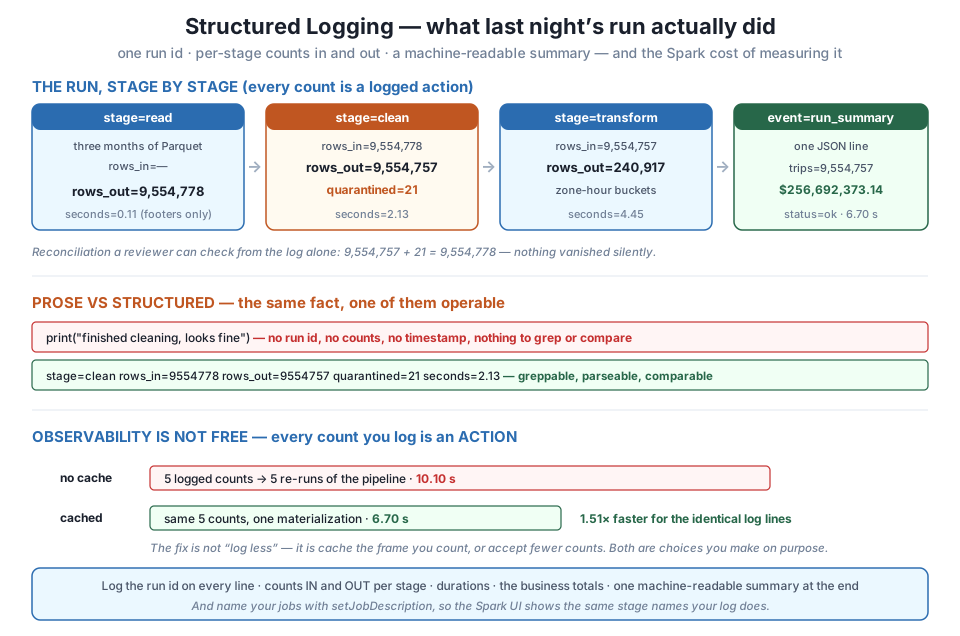
9,554,757 + 21 = 9,554,778 is checkable from the log file alone, and the run closes with one JSON line holding $256,692,373.14. The contrast panel shows why prose loses: the same event as print("finished cleaning, looks fine") carries no id, no counts, and nothing to compare against last night. The bottom panel is the honest cost — the five counts those lines require are five Spark actions, taking 10.10 s uncached against 6.70 s cached, a measured 1.51× for byte-identical output.Where these logs go in production
A FileHandler on the machine that ran the job is the starting point, not the destination. In production the same records are shipped somewhere queryable — a log aggregator, or the .jsonl summaries loaded into a small table you can join against. The reason to emit structure at the source is that this shipping step becomes trivial: key=value and JSON lines parse without a bespoke regular expression per job, so a hundred pipelines can share one ingestion path. Prose logs, by contrast, force every consumer to write a parser for one job’s phrasing, which is why they never actually get consumed.
Finally, clean up the artifacts this lesson wrote and release the session.
import os, shutil, glob
for p in glob.glob("c2m7l3_*"):
    os.remove(p)
if os.path.isdir("spark-warehouse"):
    shutil.rmtree("spark-warehouse")
spark.stop()
print("done")doneExercise 1 — Detect a bad night by diffing two summaries. The .jsonl file exists so runs can be compared. Write a compare(prev, curr) function that takes two parsed summary dicts and returns a list of warnings: flag any stage whose rows_out moved by more than 5 % between runs, and flag quarantined growing by more than 10×. Test it by hand-editing a copy of the summary to simulate a night where clean.rows_out fell to 6,000,000 and quarantined jumped to 3,554,778, and confirm your function raises both warnings.
Hint
Compute relative change as abs(curr - prev) / prev per stage and compare against your threshold; guard against a prev of zero. The two simulated numbers are chosen so that the reconciliation identity still holds — 6,000,000 + 3,554,778 does not equal 9,554,778, so a third check worth adding is that rows_out + quarantined == rows_in for the clean stage, which catches a corrupted summary that the percentage checks would let through.
Exercise 2 — Put a price on each logged count. The lesson measured all five counts together. Isolate them: time each action individually on the uncached pipeline (raw.count(), good.count(), bad.count(), report.count(), and the final agg().collect()), and rank them by cost. Then answer with numbers: if you could keep only two counts in the log, which two would you keep, and what does dropping the other three save?
Hint
Expect raw.count() to be almost free — Parquet footers, no data pages — while the two post-shuffle actions on the report dominate. Keep the counts that carry a reconciliation rather than the cheap ones: good.count() and bad.count() together prove nothing vanished, which is worth more operationally than knowing the bucket count. Remember to warm up with one full pass before timing anything.
Exercise 3 — Add a failure path to the summary. Every summary in this lesson said "status": "ok" because nothing went wrong. Wrap instrumented_run in a try/except that catches an exception, logs logger.exception(...) with the run id, and still writes a summary line — this time with "status": "failed", the stage that was in flight, and the error message. Force a failure by pointing FILES at a filename that does not exist, and confirm the .jsonl file gains a failed record that json.loads still parses.
Hint
Track the current stage name in a variable your except block can read — the stage context manager can assign it on __enter__. The discipline being practised is that a run that fails must still leave a summary; a pipeline whose logging only works on the happy path is silent exactly when you need it most. Use logger.exception rather than logger.error so the traceback lands in the file too.
You gave the pipeline a voice that survives the night. Python’s logging module was configured for a Spark job with an INFO level, a timestamped format stamping a generated run id on every line, and two handlers — stdout for a human, a file for the scheduler — with handlers.clear() and propagate = False guarding against the duplicate-line bug. Then the substance: structure over prose. stage=clean rows_in=9554778 rows_out=9554757 quarantined=21 seconds=2.13 is greppable, parseable, and comparable to last night, while "finished cleaning, looks fine" is none of those. The instrumented run logged per-stage counts in and out across the real quarter — 9,554,778 read, 9,554,757 cleaned with 21 quarantined, 240,917 zone-hour buckets carrying 9,554,757 trips and $256,692,373.14 — plus a duration per stage, and closed with one JSON line appended to a .jsonl history, which we read back with json.loads and asserted against, confirming 9,554,757 + 21 = 9,554,778 and the revenue to the cent without opening Spark. And the honest half: those five counts are five Spark actions, so logging them uncached took 10.10 s against 6.70 s cached — a measured 1.51x for identical output, concentrated in the transform stage (7.38 s to 4.45 s) where the aggregation ran twice — while read’s count was nearly free at 0.11 s because Parquet footers answer it, and caching the full nineteen-column frame instead of the three columns the job uses exhausted the driver heap outright. setJobDescription names each stage in the Spark UI with the same run id and stage string the log carries, so a slow line in the file leads straight to its shuffle in the UI.
grep retrieves exactly one night’s story.key=value pairs and JSON lines are greppable, parseable, and comparable across nights; a sentence like “looks fine” cannot be diffed against anything.rows_in, rows_out, and quarantined per stage let a reviewer verify 9,554,757 + 21 = 9,554,778 from the log alone, with no access to the data..jsonl file, is what makes “is tonight normal?” a query a monitor can run instead of a judgement a human has to make.count() in a log line re-executes the DataFrame’s recipe; uncached that cost 1.51x here, and the fix is to cache the projected frame you count or to log fewer, better-chosen counts.The value of a log is realised on exactly the days you did not plan for: the morning a dashboard looks wrong, the week a source quietly changed its schema, the incident review where someone asks what the job saw at 2 a.m. three Tuesdays ago. On those days a file full of “looks fine” is worth nothing, and a file of structured records is a complete forensic account — which stage lost rows, when it started to drift, how long it has been happening. That is why the counts are worth paying for, and why paying for them knowingly matters just as much: the same reflex that makes an engineer sprinkle count() through a job for reassurance is the one that turns a ten-minute cluster job into an hour-long one. CityFlow’s pipeline can now explain itself, and you know to the second what that explanation costs.
Your pipeline can now describe what it did, in a form both a human and a monitoring script can read. But notice what it still cannot do: stop. Every record you wrote in this lesson was status=ok, and that was true — but a job logging rows_out=6000000 on a night the source dropped a third of its data would emit that line just as calmly, write the table, exit zero, and let the morning’s dashboards publish a confidently wrong number. A log is a record, not a decision. Lesson 4, Failing Loudly, adds the judgement: thresholds that distinguish a few bad rows worth quarantining from a feed that is broken, a gate that refuses to write when a critical rule fails, and the nonzero exit code that makes a scheduler actually notice. The ordering is the whole lesson — abort before the write, so bad data is never published in the first place.
Keep DATATWEETS free. Help fund practical data, AI, and engineering lessons for learners worldwide.
