Title here
Summary here
Module 2 taught you how Spark thinks — plans, lazy evaluation, the DAG — by watching it defer work you had described. You could predict its behaviour, but you were still narrating from the sidelines. This module puts the keys in your hands: the DataFrame API is the tool CityFlow’s engineers reach for every working day, and it starts with the smallest unit of it — the column. Every filter you’ll write in Lesson 2, every join key in Lesson 3, every aggregation in Lesson 4, and the whole zone-hour report in Lesson 5 is built from column expressions. Get this one idea right and the rest of the module is composition.
And there is one idea to get right, because it trips up every engineer arriving from pandas. In pandas, df["total_amount"] hands you a Series — an actual array of 9.5 million numbers sitting in memory, which you can index, mutate, and print. In Spark, df["total_amount"] hands you something that contains no numbers at all: a Column, an expression, a description of a value to be computed later. This lesson makes that difference concrete, then cashes it in by building the derived columns CityFlow actually needs — trip duration, fare-per-mile, and pickup hour — on the real quarter. In the process you’ll meet this Spark version’s sharpest unit trap: casting a timestamp_ntz to a number to get a duration does not do what a pandas reflex expects, and getting it wrong produces a duration that is silently wrong by a factor of a million.
By the end of this lesson, you will be able to:
Column is an expression (a lazy plan node), not a list of values, and name one three ways: df["col"], F.col("col"), df.colwithColumn and select, understanding that each returns a new DataFrame and mutates nothingpyspark.sql.functions, and read the resulting dtypes from printSchema/dtypestimestamp_ntz cast trap: know that a direct cast to long fails in Spark 4, that the correct route yields seconds, and why a wrong unit is a silent bugYou’ll need pyspark with the JDK configured as in Module 1, Lesson 3, and pyspark.sql.functions, imported as F, which is the function library this whole module leans on. Start the session.
Same session shape as always — named, local, quiet — and we import the functions library right away, because everything today runs through it:
import warnings
warnings.filterwarnings("ignore")

from pyspark.sql import SparkSession
from pyspark.sql import functions as F

spark = (SparkSession.builder
         .appName("cityflow")
         .master("local[*]")
         .config("spark.ui.showConsoleProgress", "false")
         .getOrCreate())
spark.sparkContext.setLogLevel("ERROR")
print("Spark", spark.version, "-", spark.sparkContext.defaultParallelism, "task slots")
Spark 4.2.0 - 10 task slotsNow the idea to unlearn. Read the three monthly files — a plan, as Module 2 taught, so this returns instantly — and then ask what df["total_amount"] actually is, three different ways:
months = ["yellow_tripdata_2024-01.parquet",
          "yellow_tripdata_2024-02.parquet",
          "yellow_tripdata_2024-03.parquet"]
trips = spark.read.parquet(*months)

a = trips["total_amount"]
b = F.col("total_amount")
c = trips.total_amount
print("df['total_amount'] ->", type(a).__name__)
print("F.col('total_amount') ->", type(b).__name__)
print("df.total_amount ->", type(c).__name__)

expr = F.col("fare_amount") / F.col("trip_distance") + 1
print("type of an arithmetic expression:", type(expr).__name__)
print("what it prints:", expr)
df['total_amount'] -> Column
F.col('total_amount') -> Column
df.total_amount -> Column
type of an arithmetic expression: Column
what it prints: Column<'+(/(fare_amount, trip_distance), 1)'>Every one of those is a Column, and none of them contains a single value. This is the pivot the whole lesson turns on. In pandas, df["total_amount"] is the data — an array you can sum, plot, or edit in place. In Spark, df["total_amount"] is a reference to a column inside a plan — a name Spark will resolve to real numbers only when an action forces it. The three spellings are interchangeable: bracket indexing, the F.col() function, and attribute access all produce the identical Column object. (Use F.col("name") as your default — it works even when a column name collides with a DataFrame method, and it reads clearly in long expressions. Bracket form df["name"] is the other safe choice; df.name is convenient but breaks on names with spaces or dots.)
The last two lines are the real revelation. F.col("fare_amount") / F.col("trip_distance") + 1 is not a division of nine million numbers — no data has been touched. It is a new Column, and printing it shows exactly that: Column<'+(/(fare_amount, trip_distance), 1)'> — Spark’s rendering of the expression tree you just built, “add 1 to (fare_amount divided by trip_distance).” Arithmetic operators, comparisons (>, ==), and the functions in F don’t compute; they assemble expressions. A Column is a recipe for a value, in exactly the sense a DataFrame is a recipe for a table.
If a column is an expression, then handing one to select should build a plan and run nothing — the same lazy bargain from Module 2, now at the column level. Watch:
planned = trips.select((F.col("total_amount") * 2).alias("double_total"))
print("trips.select(expr) returns a", type(planned).__name__, "- nothing computed yet")
print("columns of the new frame:", planned.columns)
trips.select(expr) returns a DataFrame - nothing computed yet
columns of the new frame: ['double_total']trips.select(...) took our expression total_amount * 2, wrapped it in a plan step, and returned a new DataFrame whose single column is named — via alias — double_total. No row was doubled; planned is a description. This is why the entire lesson can build column after column and never wait: every derived column is one more node grafted onto a plan tree, and the tree isn’t evaluated until you call an action like show, count, or collect. Keep that in the back of your mind through every withColumn below — you are writing a recipe, not stirring a pot. The bill, as Module 2 measured, comes due all at once at the first action.
alias earns a note of its own: it is how you name a derived column. Without it, Spark auto-generates a name from the expression itself (the raw (total_amount * 2) string), which is ugly to reference later. Aliasing every derived column is a habit worth forming on line one.
Before deriving anything, look at what you have. A Column has a data type, and the whole DataFrame’s types are one call away:
trips.printSchema()root
|-- VendorID: integer (nullable = true)
|-- tpep_pickup_datetime: timestamp_ntz (nullable = true)
|-- tpep_dropoff_datetime: timestamp_ntz (nullable = true)
|-- passenger_count: long (nullable = true)
|-- trip_distance: double (nullable = true)
|-- RatecodeID: long (nullable = true)
|-- store_and_fwd_flag: string (nullable = true)
|-- PULocationID: integer (nullable = true)
|-- DOLocationID: integer (nullable = true)
|-- payment_type: long (nullable = true)
|-- fare_amount: double (nullable = true)
|-- extra: double (nullable = true)
|-- mta_tax: double (nullable = true)
|-- tip_amount: double (nullable = true)
|-- tolls_amount: double (nullable = true)
|-- improvement_surcharge: double (nullable = true)
|-- total_amount: double (nullable = true)
|-- congestion_surcharge: double (nullable = true)
|-- Airport_fee: double (nullable = true)printSchema() is the picture; .dtypes is the same information as a list of (name, type) tuples you can index programmatically:
print(trips.dtypes[:3], "...")
print("pickup dtype ->", dict(trips.dtypes)["tpep_pickup_datetime"])
print("dropoff dtype ->", dict(trips.dtypes)["tpep_dropoff_datetime"])
[('VendorID', 'int'), ('tpep_pickup_datetime', 'timestamp_ntz'), ('tpep_dropoff_datetime', 'timestamp_ntz')] ...
pickup dtype -> timestamp_ntz
dropoff dtype -> timestamp_ntzNote the two timestamp columns are timestamp_ntz — timestamp with no time zone, the type Module 1 flagged and Course 1’s unit trap lives inside. Under the hood these hold microsecond precision, the same as Course 1’s datetime64[us]. Money columns like total_amount are double; the location IDs are int. Knowing these types before you compute on them is not pedantry — the very next section is a bug that exists only because timestamp_ntz doesn’t behave the way a pandas reflex assumes.
CityFlow wants trip duration in minutes — dropoff time minus pickup time. The pandas reflex is to turn each timestamp into a number, subtract, and divide. In pandas you’d cast to int64 and get microseconds; here’s the direct Spark translation of that reflex. First we apply Course 1’s quarter window (so we’re working the same population everything cross-checks against), then try the naive cast:
win = trips.filter((F.col("tpep_pickup_datetime") >= "2024-01-01") &
                   (F.col("tpep_pickup_datetime") < "2024-04-01"))

try:
    bad = win.select(F.col("tpep_pickup_datetime").cast("long").alias("secs"))
    bad.show(1)
except Exception as e:
    print(type(e).__name__)
    print(str(e).splitlines()[0])
AnalysisException
[DATATYPE_MISMATCH.CAST_WITHOUT_SUGGESTION] Cannot resolve "CAST(tpep_pickup_datetime AS BIGINT)" due to data type mismatch: cannot cast "TIMESTAMP_NTZ" to "BIGINT". SQLSTATE: 42K09;(Spark also prints a longer stack trace at ERROR level around this — trimmed here to the message that matters.) So the direct route is blocked: Spark 4 refuses to cast a timestamp_ntz straight to long. That refusal is a gift — it’s the analyzer catching an ambiguity at plan time (laziness doesn’t stop type checks, as Module 2 noted) instead of letting you compute a wrong number. The reason it’s ambiguous: a zoneless timestamp has no single epoch value until you decide what zone its wall-clock reading belongs to. So you route through timestamp (a zoned instant) explicitly, and then to long:
probe = win.select(
    F.col("tpep_pickup_datetime").alias("pickup"),
    F.col("tpep_pickup_datetime").cast("timestamp").cast("long").alias("pickup_secs"),
    F.col("tpep_dropoff_datetime").cast("timestamp").cast("long").alias("dropoff_secs"),
)
probe.show(3, truncate=False)
print("dtypes:", probe.dtypes)
r = probe.first()
print("dropoff_secs - pickup_secs =", r["dropoff_secs"] - r["pickup_secs"], "for a",
      "2024-01-01 00:57:55 -> 01:17:43 trip")
+-------------------+-----------+------------+
|pickup |pickup_secs|dropoff_secs|
+-------------------+-----------+------------+
|2024-01-01 00:57:55|1704058075 |1704059263 |
|2024-01-01 00:03:00|1704054780 |1704055176 |
|2024-01-01 00:17:06|1704055626 |1704056701 |
+-------------------+-----------+------------+
only showing top 3 rows
dtypes: [('pickup', 'timestamp_ntz'), ('pickup_secs', 'bigint'), ('dropoff_secs', 'bigint')]dropoff_secs - pickup_secs = 1188 for a 2024-01-01 00:57:55 -> 01:17:43 tripNow measure the unit, because this is the whole point. The first trip ran from 00:57:55 to 01:17:43 — by the wall clock, 19 minutes 48 seconds. The casted difference is 1188. And minutes exactly. So a timestamp_ntz cast through timestamp to long yields seconds — not microseconds like Course 1’s pandas int64, and not nanoseconds. Different engine, different unit, same class of trap. Here’s why it matters, in one line:
print("as SECONDS   :", (r["dropoff_secs"] - r["pickup_secs"]) / 60, "minutes")
print("if we thought this was MICROSECONDS:", (r["dropoff_secs"] - r["pickup_secs"]) / 1e6 / 60, "minutes")
as SECONDS : 19.8 minutes
if we thought this was MICROSECONDS: 1.98e-05 minutesIf you carried Course 1’s microsecond assumption over unchanged, every trip in CityFlow’s data would clock in at two-hundred-thousandths of a minute — and nothing would crash. The pipeline would run, the report would render, and every duration would be wrong by a factor of a million. That is the definition of a silent bug, and it is exactly why the reflex to check units at every representation boundary — the reflex Course 1 drilled — has to travel with you into Spark. The unit changed; the discipline can’t.
Time zones shift the epoch, but never the difference
cast("timestamp") reads a zoneless timestamp_ntz against your session time zone to produce an instant, so the absolute pickup_secs above (1704058075) depends on that zone — a different session would print a different epoch for the same wall-clock reading. But a duration is a subtraction, and the zone offset is added to both ends and cancels: dropoff_secs - pickup_secs is 1188 in any zone. The takeaway generalizes: a difference of timestamp_ntz values is time-zone-safe, but any absolute epoch you extract from one is only as meaningful as the zone you chose. When you need the instant, be explicit about the zone; when you need the elapsed time, you’re safe.
Now bank that duration as a real column. withColumn takes a name and an expression and returns a new DataFrame with that column added — and, crucially, leaves the source frame untouched, the immutability Module 2, Lesson 4 established:
enriched = win.withColumn(
    "duration_min",
    (F.col("tpep_dropoff_datetime").cast("timestamp").cast("long") -
     F.col("tpep_pickup_datetime").cast("timestamp").cast("long")) / 60.0
)
print("win still has", len(win.columns), "columns; enriched has", len(enriched.columns))
enriched.select("tpep_pickup_datetime", "tpep_dropoff_datetime", "duration_min").show(5, truncate=False)
print("duration_min dtype:", dict(enriched.dtypes)["duration_min"])
win still has 19 columns; enriched has 20
+--------------------+---------------------+------------------+
|tpep_pickup_datetime|tpep_dropoff_datetime|duration_min |
+--------------------+---------------------+------------------+
|2024-01-01 00:57:55 |2024-01-01 01:17:43 |19.8 |
|2024-01-01 00:03:00 |2024-01-01 00:09:36 |6.6 |
|2024-01-01 00:17:06 |2024-01-01 00:35:01 |17.916666666666668|
|2024-01-01 00:36:38 |2024-01-01 00:44:56 |8.3 |
|2024-01-01 00:46:51 |2024-01-01 00:52:57 |6.1 |
+--------------------+---------------------+------------------+
only showing top 5 rows
duration_min dtype: doubleTwo things to read here. First, immutability: win still reports 19 columns while enriched has 20 — withColumn didn’t modify win, it returned a new plan that describes win plus one derived column. (If you pass withColumn a name that already exists, it replaces that column instead of adding one — same call, and still a new frame either way.) Second, the dtype is double, because we divided by 60.0; the first trip reads 19.8 minutes, matching the hand-check exactly, and the rest are believable New York cab rides.
There’s a cleaner idiom worth knowing, too: subtract the two timestamp_ntz columns directly and Spark hands you an interval type, no casting at all:
interval = win.select(
    (F.col("tpep_dropoff_datetime") - F.col("tpep_pickup_datetime")).alias("duration")
)
interval.show(3, truncate=False)
print("duration dtype:", interval.dtypes)
+-----------------------------------+
|duration |
+-----------------------------------+
|INTERVAL '0 00:19:48' DAY TO SECOND|
|INTERVAL '0 00:06:36' DAY TO SECOND|
|INTERVAL '0 00:17:55' DAY TO SECOND|
+-----------------------------------+
only showing top 3 rows
duration dtype: [('duration', 'interval day to second')]INTERVAL '0 00:19:48' is the same first trip — 19 minutes 48 seconds — read straight off, no unit trap possible because Spark tracks the unit for you. The interval is the more honest representation; the divide-by-60 double is the more convenient one for later math and aggregation. Both are correct now that you know the seconds fact underneath.
Two more derived columns, chained onto enriched. Fare-per-mile is plain arithmetic on two double columns, wrapped in F.round for readability; pickup hour uses the date function F.hour, which pulls the hour-of-day out of a timestamp:
enriched = (enriched
    .withColumn("fare_per_mile", F.round(F.col("total_amount") / F.col("trip_distance"), 2))
    .withColumn("pickup_hour", F.hour("tpep_pickup_datetime")))
enriched.select("total_amount", "trip_distance", "fare_per_mile",
                "tpep_pickup_datetime", "pickup_hour").show(5, truncate=False)
print("fare_per_mile dtype:", dict(enriched.dtypes)["fare_per_mile"],
      "| pickup_hour dtype:", dict(enriched.dtypes)["pickup_hour"])
+------------+-------------+-------------+--------------------+-----------+
|total_amount|trip_distance|fare_per_mile|tpep_pickup_datetime|pickup_hour|
+------------+-------------+-------------+--------------------+-----------+
|22.7 |1.72 |13.2 |2024-01-01 00:57:55 |0 |
|18.75 |1.8 |10.42 |2024-01-01 00:03:00 |0 |
|31.3 |4.7 |6.66 |2024-01-01 00:17:06 |0 |
|17.0 |1.4 |12.14 |2024-01-01 00:36:38 |0 |
|16.1 |0.8 |20.13 |2024-01-01 00:46:51 |0 |
+------------+-------------+-------------+--------------------+-----------+
only showing top 5 rows
fare_per_mile dtype: double | pickup_hour dtype: intThe first trip paid $22.70 all-in over 1.72 miles — $13.20 per mile, a plausible short-hop Manhattan rate (short trips carry the fixed base fare over few miles, so their per-mile rate runs high; the $6.66 on the 4.7-mile trip is the more efficient long ride). All five pickups fall in hour 0 — the post-midnight hour of January 1, which is exactly where the file’s first rows live. One honest caveat carried forward to Lesson 2: trip_distance has real dirt in it (Course 1 measured a maximum of 312,722 miles), and dividing by a zero or absurd distance would give Infinity or a meaningless rate — cleaning that is Lesson 2’s job, not this one’s.
F.hour is one of dozens of functions in pyspark.sql.functions. It’s worth seeing the date family beside its cousin F.date_trunc, because they answer different questions — one gives you the hour number, the other gives you the hour bucket (the timestamp floored to the hour), which is what the zone-hour report groups on:
buckets = win.select(
    F.col("tpep_pickup_datetime").alias("pickup"),
    F.hour("tpep_pickup_datetime").alias("hour_of_day"),
    F.date_trunc("hour", "tpep_pickup_datetime").alias("hour_bucket"),
    F.dayofweek("tpep_pickup_datetime").alias("dow"),
)
buckets.show(3, truncate=False)
print("dtypes:", buckets.dtypes)
+-------------------+-----------+-------------------+---+
|pickup |hour_of_day|hour_bucket |dow|
+-------------------+-----------+-------------------+---+
|2024-01-01 00:57:55|0 |2024-01-01 00:00:00|2 |
|2024-01-01 00:03:00|0 |2024-01-01 00:00:00|2 |
|2024-01-01 00:17:06|0 |2024-01-01 00:00:00|2 |
+-------------------+-----------+-------------------+---+
only showing top 3 rows
dtypes: [('pickup', 'timestamp_ntz'), ('hour_of_day', 'int'), ('hour_bucket', 'timestamp'), ('dow', 'int')]hour_of_day is an int (0–23); hour_bucket is a timestamp floored to :00:00; dow is the day of week where Spark numbers Sunday as 1, so 2 here is Monday — correct, January 1, 2024 was a Monday. The string family works the same way. Here it is on the zone dimension you’ll join in Lesson 3, showing three common string functions at once:
zones = spark.read.option("header", True).csv("taxi_zone_lookup.csv")
zones.select(
    F.col("Zone"),
    F.upper("Zone").alias("upper"),
    F.substring("Zone", 1, 4).alias("first4"),
    F.concat_ws(" / ", "Borough", "Zone").alias("label"),
).show(4, truncate=False)
+-----------------------+-----------------------+------+-------------------------------+
|Zone |upper |first4|label |
+-----------------------+-----------------------+------+-------------------------------+
|Newark Airport |NEWARK AIRPORT |Newa |EWR / Newark Airport |
|Jamaica Bay |JAMAICA BAY |Jama |Queens / Jamaica Bay |
|Allerton/Pelham Gardens|ALLERTON/PELHAM GARDENS|Alle |Bronx / Allerton/Pelham Gardens|
|Alphabet City |ALPHABET CITY |Alph |Manhattan / Alphabet City |
+-----------------------+-----------------------+------+-------------------------------+
only showing top 4 rowsF.upper uppercases, F.substring slices (1-indexed, so 1, 4 is the first four characters), and F.concat_ws joins with a separator. Every one is a Column-in, Column-out expression — the same lazy building blocks, just for text.
Prefer built-in F.* functions over Python UDFs
You could write any of these derivations as a Python UDF — a plain function wrapped with F.udf — and sometimes you must, for logic the library can’t express. Prefer the built-in F.* functions whenever they’ll do the job. The reason is the one Module 2 measured for RDD lambdas: a UDF is opaque Python that Catalyst can’t see into or optimize, and every row crosses the JVM-to-Python boundary to reach it. A built-in like F.hour stays inside the JVM as an expression the optimizer understands. Module 4 puts a number on that gap; here, just build the reflex — reach for F first, and drop to a UDF only when F genuinely can’t express what you need.
A derived column that looks right isn’t verified until it matches something you already trust. You built pickup_hour and the hour_bucket; Course 1 and Module 2 both established the quarter’s single busiest zone-hour. So group the buckets by zone and hour, count, and sort — the same shape Lesson 4 will formalize — and see whether the derivation lands on the known answer:
report = (win
    .withColumn("hour_bucket", F.date_trunc("hour", "tpep_pickup_datetime"))
    .groupBy("PULocationID", "hour_bucket")
    .agg(F.count("*").alias("trips"))
    .orderBy(F.col("trips").desc()))
report.show(3, truncate=False)
+------------+-------------------+-----+
|PULocationID|hour_bucket |trips|
+------------+-------------------+-----+
|79 |2024-02-25 01:00:00|846 |
|79 |2024-02-25 00:00:00|803 |
|161 |2024-02-29 17:00:00|779 |
+------------+-------------------+-----+
only showing top 3 rowsThe busiest zone-hour in the whole quarter is zone 79 at 2024-02-25 01:00:00 with 846 trips — the exact bucket Module 2’s report surfaced and Course 1 verified. Zone 79 is East Village, and the top three buckets are all its late-night hours (1 a.m. and midnight, plus a Midtown Center rush hour on leap day). One last confirmation, that this really is a Sunday-night bar-close pattern:
peak = spark.createDataFrame([("2024-02-25 01:00:00",)], ["t"]).select(
    F.to_timestamp("t").alias("t"),
    F.date_format(F.to_timestamp("t"), "EEEE").alias("weekday"))
peak.show(truncate=False)
+-------------------+-------+
|t |weekday|
+-------------------+-------+
|2024-02-25 01:00:00|Sunday |
+-------------------+-------+Sunday. Your date_trunc-derived hour, grouped and counted from scratch, reproduces the audited answer to the trip — East Village, 1 a.m. Sunday, 846 pickups. That is what it means for a derived column to be correct rather than merely plausible: it agrees with ground truth you established independently. The cross-verification habit that made Module 2 trustworthy carries straight into column work.
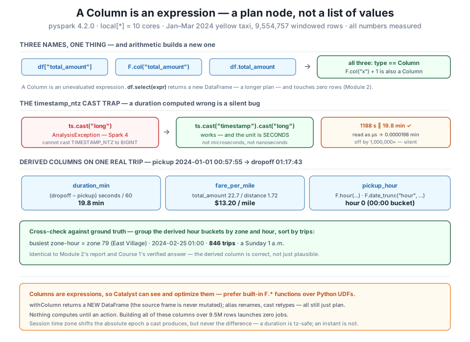
Column is an expression, not data. All three ways of naming a column return a Column, and arithmetic on them builds a new one — a lazy plan node that computes nothing until an action. The timestamp_ntz cast trap: a direct cast("long") raises an AnalysisException, the correct route through timestamp yields seconds, and the first trip's 1188 s is 19.8 min — read as microseconds it would be off by 1,000,000×, silently. The derived hour cross-checks to ground truth: busiest zone-hour is zone 79 (East Village), Sunday 1 a.m. Feb 25, 846 trips, matching Course 1 exactly.The session’s work is done — release it:
spark.stop()
print("session stopped")
session stoppedExercise 1 — Name it three ways, prove it’s one thing. For the total_amount column, build the same expression — say, total_amount * 0.9 (a 10% discount) — three times, once using df["total_amount"], once using F.col("total_amount"), and once using df.total_amount. Confirm all three are Column objects with type(...).__name__, then use each to build a select and check that the three resulting DataFrames have identical schemas. Finally, print one of the expressions directly (not inside a select) and read the expression tree Spark shows you.
Hint
All three spellings resolve to the identical Column, so all three selects produce the same one-column plan — type(...).__name__ returns Column every time, and the schemas match. Printing F.col("total_amount") * 0.9 shows something like Column<'*(total_amount, 0.9)'> — the expression tree, not a number, because nothing has run. If you’re tempted to also call an action to “see the values,” resist: the point of the exercise is that you can build and inspect the whole thing with zero jobs launched.
Exercise 2 — Re-derive duration two ways and reconcile them. Take the windowed frame and compute trip duration two ways: (a) the cast("timestamp").cast("long") difference divided by 60, and (b) the direct timestamp subtraction that yields an interval. Show the first five rows of each side by side. Do they describe the same durations? Then answer in one sentence: why does the direct cast("long") on the raw timestamp_ntz — without the intermediate cast("timestamp") — fail?
Hint
They must agree: the first trip is 19.8 minutes as a double and INTERVAL '0 00:19:48' as an interval — same 19 minutes 48 seconds, two representations. The direct cast("long") fails with DATATYPE_MISMATCH.CAST_WITHOUT_SUGGESTION because a timestamp_ntz has no time zone, so Spark can’t decide which epoch second it corresponds to without you first pinning it to a zoned timestamp. If your two methods disagree, check that you divided the seconds difference by 60 and not 60.0 inside integer arithmetic somewhere, or that you didn’t accidentally swap pickup and dropoff.
Exercise 3 — A derived weekday, cross-checked. Add a pickup_weekday column using F.date_format(..., "EEEE") (the full weekday name) and a pickup_hour column with F.hour. Then, without grouping by zone this time, group only by pickup_weekday and pickup_hour, count, and find the single busiest weekday-hour across the whole quarter. Which day and hour win, and does the winner make sense against the East Village Sunday-1-a.m. pattern you saw in the lesson?
Hint
Collapsing away the zone aggregates all pickups everywhere into weekday-hour buckets, so the winner reflects citywide rhythm, not one nightlife zone — expect a busy weekday commuting or evening hour to top it rather than Sunday 1 a.m. (that bucket was the busiest zone-hour, a much narrower slice). The lesson’s peak was one zone at one timestamp; this is every zone summed by clock pattern, so a different answer is the correct answer, not a contradiction — reason about why before you run it. Use F.dayofweek if you’d rather sort numerically, but date_format(..., "EEEE") gives you the readable name for the final answer.
A Spark Column is an expression, not a list of values — the single idea this lesson exists to install. df["total_amount"], F.col("total_amount"), and df.total_amount all return the identical Column, and arithmetic or comparisons on them build new columns: type(F.col("fare_amount") / F.col("trip_distance") + 1) is Column, printing as an expression tree, having touched zero rows. Handing an expression to select or withColumn grows a plan and returns a new DataFrame — win kept its 19 columns while enriched gained a 20th — so column work is as lazy as everything in Module 2. On the real quarter you derived three columns CityFlow needs: trip duration, defusing this version’s sharpest trap along the way — a direct cast("long") on a timestamp_ntz raises an AnalysisException, the correct route through timestamp yields seconds, and the first trip’s 1188-second gap is 19.8 minutes, versus the 0.0000198 minutes a microsecond misreading would silently produce; fare-per-mile ($13.20 on that first short hop); and pickup hour via F.hour and F.date_trunc. printSchema/dtypes confirmed the timestamps are timestamp_ntz and the derived types (double, int, timestamp, interval) came out as expected. Finally the derived hour cross-checked to ground truth: grouped by zone and hour, the busiest bucket is zone 79 — East Village — at 1 a.m. on Sunday, February 25, with 846 trips, exactly Course 1’s verified answer.
Column as expression — a lazy plan node describing a value, not an array of values; named three interchangeable ways (df["c"], F.col("c"), df.c), combined with operators and F.* functions into new columns, and evaluated only at an action.select vs withColumn — both return a new DataFrame and mutate nothing (win stayed 19 columns, enriched became 20). withColumn(name, expr) adds or replaces one named column; alias names a derived column, cast retypes it.timestamp_ntz cast trap — direct cast("long") fails in Spark 4 (DATATYPE_MISMATCH); routing through timestamp yields seconds, so a duration is secondsdiff / 60, and assuming microseconds makes it wrong by 1,000,000× without any error.F) — pyspark.sql.functions supplies arithmetic, string (upper, substring, concat_ws), and date (hour, dayofweek, date_trunc, date_format) expressions; prefer these built-ins over Python UDFs because Catalyst can optimize them and they never cross the JVM-to-Python boundary per row.date_trunc hour, grouped and counted, lands on zone 79 / Sunday 1 a.m. / 846 trips, matching Course 1.Every transformation CityFlow’s engineers write for the rest of this course is column expressions composed together — the filters of Lesson 2, the join keys of Lesson 3, the aggregations of Lesson 4, the whole report of Lesson 5. An engineer who still pictures a Spark column as a pandas Series will fight the API at every turn: they’ll try to iterate it, index into it, mutate it in place, and wonder why none of that works — because there are no values there to touch, only a plan waiting to be run. And the timestamp_ntz trap is the kind of bug that survives code review and ships, precisely because it doesn’t crash: a duration column silently scaled by a million passes every “does it run” check and quietly corrupts every downstream metric that touches trip time. The habit that catches it is not Spark-specific — it’s the units-and-boundaries discipline Course 1 built, now proven to matter just as much in a new engine with a new unit. Derive carefully, check the dtype, and cross-verify against something you already trust, and your columns will be correct rather than merely plausible.
You can now build any derived column you need, and you know the difference between one that’s correct and one that merely runs. But the taxi quarter you’ve been deriving on is still dirty — the same real defects Course 1 catalogued are all still in there, hiding under those clean-looking first rows: timestamps from 2002 and 2009 that the window quietly quarantines, tens of thousands of negative fares that are accounting reversals rather than errors, and trip distances up to 312,722 miles. Lesson 2, Filtering & Cleaning, is where you confront that dirt in Spark and — this is the part that separates a careful engineer from a careless one — learn what not to delete. You’ll use filter, where, isNull, between, and when/otherwise to clean the data, and you’ll measure the trap at the center of it: a filter that drops the negative fares looks like tidying up and actually overstates revenue by a measured six figures a month, because those reversals must stay in the data for the totals to balance. The columns you built today are the vocabulary; cleaning is the judgment that keeps them honest.
Keep DATATWEETS free. Help fund practical data, AI, and engineering lessons for learners worldwide.
