Title here
Summary here
Lesson 1 gave you the Column object: select, withColumn, expressions, casts. You can now shape a DataFrame. This lesson is about shrinking one — deciding which rows deserve to survive — and it is the most dangerous thing CityFlow’s engineers do all quarter. Filtering feels innocent. You write filter(total_amount >= 0) because negative money “looks wrong,” the count drops a little, the code turns green, and you have just fabricated three million dollars of revenue that never existed. The taxi data is genuinely dirty — a pickup stamped in 2002, a single trip logged at 312,722 miles, three quarters of a million rows with missing passenger counts — and the engineer’s whole job is telling dirt apart from data that merely offends a tidy instinct. Get that judgment wrong and every downstream number inherits the mistake.
So this lesson is not a syntax tour, though you will meet every filtering tool Spark has. It is a lesson in restraint, measured on the real quarter. You will apply the quarter window and watch it quarantine exactly 21 rows — not the 56 you might expect, and the gap between those numbers is itself a lesson. You will count the 115,894 negative-total_amount rows, prove with a SUM that they are accounting reversals rather than errors, and then deliberately do the wrong thing — drop them — and measure the $2,986,808.76 of phantom revenue that appears. You will flag a 312,722-mile trip without deleting it, and fill 751,962 nulls instead of dropping the trips that carry them. Every number here is real, and the ones that hurt are the point.
By the end of this lesson, you will be able to:
filter/where, boolean Column expressions, and the & / | / ~ operators (with the parentheses Python forces on you)isNull, isNotNull, isin, between, and rlike to express real cleaning conditions, and audit which columns are actually dirty before touching themwhen/otherwise to flag rather than delete — measured on trip_distance’s 312,722-mile maxna.drop and na.fill on the 751,962 rows with missing values, and explain why the choice changes CityFlow’s trip count but not its revenueYou’ll need pyspark with the JDK configured as in Module 1, Lesson 3. Start the session.
Filtering in Spark is deliberately dull, and that is a feature. filter and where are the same method — where is a SQL-friendly alias, byte-for-byte identical, pick whichever reads better. Both take a boolean Column expression: an expression like F.col("trip_distance") > 100 that, evaluated per row, produces True or False. It is lazy, exactly like every expression in Lesson 1 — it builds a plan node, touches no data — until an action forces it.
Start the session and build one such expression without running it, to make the laziness concrete:
import warnings
warnings.filterwarnings("ignore")

from pyspark.sql import SparkSession
from pyspark.sql import functions as F

spark = (SparkSession.builder
         .appName("cityflow")
         .master("local[*]")
         .config("spark.ui.showConsoleProgress", "false")
         .getOrCreate())
spark.sparkContext.setLogLevel("ERROR")

months = ["yellow_tripdata_2024-01.parquet",
          "yellow_tripdata_2024-02.parquet",
          "yellow_tripdata_2024-03.parquet"]
trips = spark.read.parquet(*months)

long_trips = F.col("trip_distance") > 100
print("a condition is a", type(long_trips).__name__, "- no rows touched yet")
print(long_trips)
a condition is a Column - no rows touched yet
Column<'(trip_distance > 100)'>The condition is a Column, printable, inert. Now the operators, because they are the one place Spark’s filtering bites Python users. You cannot write a and b or not a on Columns — Python’s keyword operators can’t be overloaded, and Spark hijacks the bitwise ones instead: & for AND, | for OR, ~ for NOT. And because & binds tighter than >, every comparison must be wrapped in its own parentheses or the expression parses into nonsense. This is the single most common Spark filtering bug; burn the parentheses into muscle memory:
# gate: skip
# The AND / OR / NOT operators on Columns - parentheses are mandatory:
in_window = (F.col("tpep_pickup_datetime") >= "2024-01-01") & \
            (F.col("tpep_pickup_datetime") <  "2024-04-01")
short_or_far = (F.col("trip_distance") < 0.1) | (F.col("trip_distance") > 100)
not_cash     = ~F.col("payment_type").isin(1, 2)
#   &  = AND      |  = OR      ~  = NOT
#   WRONG:  F.col("x") > 1 & F.col("y") < 2   ->  parses as x > (1 & y) < 2
The rest of the toolkit is a short vocabulary you’ll use for the whole lesson, each one a Column method that returns a boolean Column: isNull() and isNotNull() for missing values; isin(a, b, c) for set membership; between(lo, hi) for inclusive ranges; like("%JFK%") for SQL wildcards and rlike(...) for full regular expressions; when(cond, x).otherwise(y) to build a new column by cases rather than filtering rows away; and the df.na family — na.fill, na.drop, na.replace — for missing data. We’ll meet each on real dirt. But first, the filter that every CityFlow report begins with.
Course 1 established the golden rule: before you count anything, restrict the data to the quarter you actually mean — pickups on or after 2024-01-01 and strictly before 2024-04-01. It sounds like bookkeeping. It is really a data-integrity filter, because the monthly files are not clean calendar months. Count the raw quarter, then the windowed quarter, and read the gap:
raw = trips.count()

window = ((F.col("tpep_pickup_datetime") >= "2024-01-01") &
          (F.col("tpep_pickup_datetime") <  "2024-04-01"))
tw = trips.filter(window)
kept = tw.count()

print(f"raw three-file quarter : {raw:,}")
print(f"after the window filter : {kept:,}")
print(f"quarantined by the window: {raw - kept:,}")
raw three-file quarter : 9,554,778
after the window filter : 9,554,757
quarantined by the window: 219,554,778 raw, 9,554,757 kept, 21 removed — and that 21 is Course 1’s verified quarantine count, reproduced in Spark on the first try. But 21 is a strange number, because the files contain more than 21 misfiled rows. Each monthly file should hold only its own month; count the rows in each file whose pickup falls outside that file’s own month, and a different number appears:
files = [("yellow_tripdata_2024-01.parquet", "2024-01-01", "2024-02-01", "Jan"),
         ("yellow_tripdata_2024-02.parquet", "2024-02-01", "2024-03-01", "Feb"),
         ("yellow_tripdata_2024-03.parquet", "2024-03-01", "2024-04-01", "Mar")]

total = 0
for path, lo, hi, label in files:
    f = spark.read.parquet(path)
    own = f.filter((F.col("tpep_pickup_datetime") >= lo) &
                   (F.col("tpep_pickup_datetime") <  hi)).count()
    strays = f.count() - own
    total += strays
    print(f"{label} file: {strays} rows outside its own month")
print(f"total per-file strays: {total}")
Jan file: 18 rows outside its own month
Feb file: 15 rows outside its own month
Mar file: 23 rows outside its own month
total per-file strays: 5656 per-file strays, but only 21 quarantined. The other 35 are month-boundary spill: a trip picked up at 2024-02-01 00:01 that the vendor happened to write into the January file, or a February pickup logged in March. Those 35 rows are misfiled relative to their file, but they are still inside the quarter, so the quarter window correctly keeps them — they are real Q1 trips. Only the 21 rows that fall outside the quarter entirely get removed. This is why the FILES and the WINDOW are two different populations, and why every cross-check in this course applies the window first: a raw per-file count and a windowed report disagree by exactly these strays.
The 21 quarantined rows are not near the boundary — they are wild. A filter surfaces the worst of them:
mar = spark.read.parquet("yellow_tripdata_2024-03.parquet")
(mar.filter(F.col("tpep_pickup_datetime") < "2024-01-01")
    .select("tpep_pickup_datetime", "tpep_dropoff_datetime",
            "PULocationID", "total_amount")
    .orderBy(F.col("tpep_pickup_datetime").asc())
    .show(truncate=False))
+--------------------+---------------------+------------+------------+
|tpep_pickup_datetime|tpep_dropoff_datetime|PULocationID|total_amount|
+--------------------+---------------------+------------+------------+
|2002-12-31 22:17:10 |2002-12-31 22:42:24 |50 |18.0 |
|2002-12-31 23:08:30 |2003-01-01 14:58:35 |132 |25.15 |
+--------------------+---------------------+------------+------------+The quarter’s earliest stray is a pickup stamped 2002-12-31 22:17:10 — twenty-one years before the data it sits inside — hiding in the March file, of all places. It is not a February-into-January spill you could rationalize; it is a meter clock that was never set, or a replayed test record. The window filter removes it and the twenty like it, silently and correctly, because “a trip from 2002” is not part of the Q1 2024 population no matter how you squint. This is the one place in the lesson where deleting rows is unambiguously right: you are not judging the rows bad, you are defining the population you meant to study. Everything after this is harder.
Here is the row that fools everyone. Some trips have a negative total_amount. To an engineer trained on “clean your data,” a negative fare is obviously garbage — money can’t be negative — so the reflex is filter(F.col("total_amount") >= 0) and move on. Count them first:
neg = tw.filter(F.col("total_amount") < 0).count()
zero = tw.filter(F.col("total_amount") == 0).count()
pos = tw.filter(F.col("total_amount") > 0).count()
print(f"in-window trips with total_amount < 0 : {neg:,}")
print(f"                          == 0        : {zero:,}")
print(f"                          >  0        : {pos:,}")
in-window trips with total_amount < 0 : 115,894
== 0 : 1,292
> 0 : 9,437,571115,894 negative rows — not a handful of glitches, over one percent of the quarter. That volume alone should stop your hand: real errors are rare and random; 115,894 systematic negatives are a category. Look at a few:
(tw.filter(F.col("total_amount") < 0)
   .select("tpep_pickup_datetime", "PULocationID",
           "payment_type", "fare_amount", "total_amount")
   .orderBy(F.col("tpep_pickup_datetime").asc(), F.col("PULocationID").asc())
   .show(5, truncate=False))
+--------------------+------------+------------+-----------+------------+
|tpep_pickup_datetime|PULocationID|payment_type|fare_amount|total_amount|
+--------------------+------------+------------+-----------+------------+
|2024-01-01 00:04:00 |63 |2 |-31.5 |-34.25 |
|2024-01-01 00:05:38 |140 |4 |-5.1 |-10.1 |
|2024-01-01 00:07:37 |114 |4 |-3.0 |-8.0 |
|2024-01-01 00:07:49 |158 |4 |-7.2 |-12.2 |
|2024-01-01 00:08:26 |234 |3 |-3.0 |-5.5 |
+--------------------+------------+------------+-----------+------------+
only showing top 5 rowsEvery component is negative — the fare, the total, the surcharges — a mirror image of a normal trip. These are reversals: a charge that was billed, then voided, then usually re-billed correctly. Course 1 proved this by matching each negative row to a positive twin with the same trip key; the negative is the accounting undo of a duplicate charge. The vendor leaves both the original charge and its reversal in the data on purpose, because that is how a ledger stays auditable — you don’t erase a mistake, you post an offsetting entry. The taxi feed is a ledger, and total_amount is designed so that SUM lets the pairs cancel.
Which means dropping the negatives doesn’t remove errors — it removes half of every reversal pair, leaving the erroneous original charge behind with nothing to cancel it. Measure the damage directly. Sum the revenue with the reversals kept, then sum it again with them dropped:
rev_keep = tw.agg(F.sum("total_amount")).first()[0]
rev_drop = (tw.filter(F.col("total_amount") >= 0)
              .agg(F.sum("total_amount")).first()[0])

print(f"revenue KEEPING the reversals : ${rev_keep:,.2f}")
print(f"revenue DROPPING the reversals: ${rev_drop:,.2f}")
print(f"phantom revenue introduced    : ${rev_drop - rev_keep:,.2f}")
revenue KEEPING the reversals : $256,692,373.14
revenue DROPPING the reversals: $259,679,181.90
phantom revenue introduced : $2,986,808.76Read those three lines slowly, because they are the whole lesson. Keeping the reversals gives $256,692,373.14 — Course 1’s verified quarter revenue, to the cent, because the offsetting entries did their job. Dropping them gives $259,679,181.90: the “clean” pipeline reports $2,986,808.76 more revenue than CityFlow actually earned. Not a rounding wobble — nearly three million dollars of income invented by a one-line filter that felt like hygiene. The distortion scales with volume, too — split by month, dropping the reversals overstates January by , February by , and March by , the same order of magnitude Course 1 measured for the reversal swing.
The rule, then, is inverted from instinct: a negative total_amount is the most trustworthy row in the file, not the least. It is an explicit correction. You keep it precisely because it is accounting, and you let SUM do what SUM was built to do. The only cleaning a reversal ever needs is the window filter it already passed.
“Clean” is not a synonym for “positive”
The trap here is linguistic as much as technical. “Clean the data” gets silently rewritten in your head as “remove the rows that look unusual,” and negative money looks unusual. But unusual and wrong are different claims, and only measurement can tell them apart. The discipline: before you filter a row out, state the specific error you believe it represents, then check whether removing it makes a known-good number better or worse. Here, dropping the negatives made a number Course 1 had already verified to the cent get worse by $2,986,808.76 — proof, not opinion, that the filter was the bug.
Not every dirty value is secretly correct. trip_distance really does contain nonsense — find its maximum:
dist = tw.agg(F.max("trip_distance").alias("max"),
              F.min("trip_distance").alias("min")).first()
print(f"max trip_distance: {dist['max']:,.1f} miles")
print(f"min trip_distance: {dist['min']:,.1f} miles")
print("trips over 100 mi :", f"{tw.filter(F.col('trip_distance') > 100).count():,}")
print("trips at exactly 0:", f"{tw.filter(F.col('trip_distance') == 0).count():,}")
max trip_distance: 312,722.3 miles
min trip_distance: 0.0 miles
trips over 100 mi : 252
trips at exactly 0: 215,764312,722 miles in a New York taxi is a broken meter — that is farther than a round trip to the Moon, inside a five-borough fare. This value is genuinely wrong, unlike the negatives. But that does not license filter(F.col("trip_distance") < 100), and the reason is the 215,764 rows at exactly zero: a 0.0-mile trip is often a real, legitimate record — a fare that was cancelled at the curb, a minimum-charge airport wait, a meter that logged time but no motion. Some analyses want those; some don’t. If your filter deletes rows to protect your current question, the next engineer inherits a dataset that silently can’t answer theirs.
So flag instead of delete. when/otherwise builds a new column by cases — Spark’s vectorized if/elif/else — leaving every row in place with a label that downstream code can honor or ignore:
flagged = tw.withColumn(
    "distance_flag",
    F.when(F.col("trip_distance") > 100, "suspect")
     .when(F.col("trip_distance") == 0, "zero")
     .otherwise("ok"))

flagged.groupBy("distance_flag").count().orderBy("distance_flag").show()
+-------------+-------+
|distance_flag| count|
+-------------+-------+
| ok|9338741|
| suspect| 252|
| zero| 215764|
+-------------+-------+Now the data carries its own verdict. The 252 suspect trips over 100 miles and the 215,764 zero-mile trips are labelled, not gone; a revenue report can keep them all (they still paid), a trip-length analysis can filter(distance_flag == "ok") for itself, and no one has to re-derive which rows were dubious because the column remembers. The 9,338,741 ok trips are untouched. This is the general shape of honest cleaning: when/otherwise adds knowledge; filter removes rows — reach for the first unless you are certain the rows have no business existing at all.
You could go further and cap rather than flag — F.when(F.col("trip_distance") > 100, 100).otherwise(F.col("trip_distance")) to winsorize the outliers for a model — and that is a legitimate choice too, as long as it is a labelled, reversible transformation on a copy and not a silent overwrite of the source. The engineering principle is the same either way: transformations that change the data must announce themselves.
Missing data is the last kind of dirt, and the first question is never “how do I handle nulls” — it is “which columns actually have any.” Guessing wastes effort cleaning clean columns and, worse, invites a blanket na.drop() that deletes far more than you think. Audit all nineteen columns at once by summing a null-indicator per column:
exprs = [F.sum(F.col(c).isNull().cast("int")).alias(c) for c in trips.columns]
audit = tw.agg(*exprs).first().asDict()
dirty = {c: n for c, n in audit.items() if n > 0}
for c, n in dirty.items():
    print(f"{c:>22}: {n:,} nulls")
print("all other columns: 0 nulls")
passenger_count: 751,962 nulls
RatecodeID: 751,962 nulls
store_and_fwd_flag: 751,962 nulls
congestion_surcharge: 751,962 nulls
Airport_fee: 751,962 nulls
all other columns: 0 nullsFive columns, and every one reports the identical 751,962. That is not a coincidence — it is a signature. The same 751,962 rows are null in all five columns at once; confirm it:
all_five_null = tw.filter(
    F.col("passenger_count").isNull() &
    F.col("RatecodeID").isNull() &
    F.col("store_and_fwd_flag").isNull() &
    F.col("congestion_surcharge").isNull() &
    F.col("Airport_fee").isNull()).count()
print(f"rows null in ALL FIVE columns at once: {all_five_null:,}")
print(f"share of the quarter: {all_five_null / kept * 100:.2f}%")
rows null in ALL FIVE columns at once: 751,962
share of the quarter: 7.87%All 751,962 nulls are co-located in the same rows — 7.87% of the quarter. These are trips a subset of vendors reported with a leaner schema: no passenger count, no rate code, no airport fee. Critically, their total_amount, PULocationID, and timestamps are all present and valid. They are complete trips with incomplete metadata. Now the fork that decides whether your counts survive. The blunt tool is na.drop(), which deletes any row with a null in any column:
after_drop = tw.na.drop().count()
print(f"trips before na.drop(): {kept:,}")
print(f"trips after  na.drop(): {after_drop:,}")
print(f"real trips deleted    : {kept - after_drop:,}")
trips before na.drop(): 9,554,757
trips after na.drop(): 8,802,795
real trips deleted : 751,962A single na.drop() erased 751,962 real trips — every fare, every dollar of their revenue, every pickup — because their passenger count was blank. Any “how many trips did CityFlow serve” question now answers 8,802,795 instead of 9,554,757: an 8% undercount born of one method call. The right tool when the row is real but a field is missing is na.fill, which keeps the row and supplies a placeholder you can recognize later:
filled = tw.na.fill({"passenger_count": 0, "RatecodeID": 99})
still_here = filled.count()
sentinel = filled.filter(F.col("passenger_count") == 0).count()
print(f"trips after na.fill(): {still_here:,}  (none deleted)")
print(f"rows now carrying the passenger_count=0 sentinel: {sentinel:,}")
trips after na.fill(): 9,554,757 (none deleted)
rows now carrying the passenger_count=0 sentinel: 105,931Every trip survives, and the fill is honest: filling passenger_count with 0 folds the 751,962 unknowns in with the 105,931 rows that already logged zero passengers, so a placeholder of 99 or a separate passenger_known boolean is often the more truthful choice — the point is that the decision is yours to make deliberately, not na.drop()’s to make for you by deletion. The judgment throughout: na.drop changes your trip count; na.fill changes only a field. A missing passenger count is not a missing trip, and no cleaning step should confuse the two.
dropDuplicates has the same reversal trap
dropDuplicates() with no arguments removes only fully identical rows — Course 1 found just 2 of those in the whole quarter, both in February — which is safe. The danger is dropDuplicates(subset=[...key columns...]), which keeps one row per key and deletes the rest. Run it on the trip-identifying columns and it collapses every reversal pair back into a single row, deleting exactly the offsetting entries you just learned to protect — reintroducing the $2,986,808.76 error through a different door. “Deduplicate on a subset” is the same mistake as “drop the negatives,” wearing a different name. Deduplicate on the whole row, or not at all, unless you have proven the subset is a true unique key.
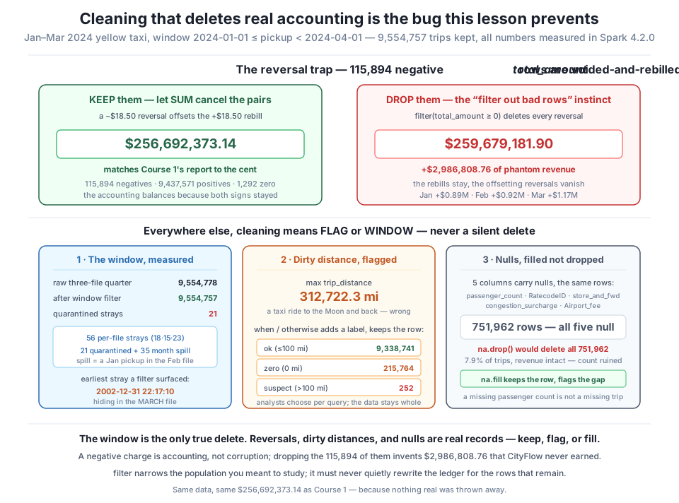
2002-12-31 22:17:10 in the March file. The other three are traps: dropping the 115,894 negative-total_amount reversals overstates revenue by $2,986,808.76 because SUM was built to let them cancel to Course 1's $256,692,373.14; the 312,722-mile trip_distance is flagged with when/otherwise, not deleted; and the 751,962 rows with five co-located nulls are filled, not dropped — na.drop() would erase 7.9% of real trips. filter narrows the population you meant to study; it must never quietly rewrite the ledger for the rows that remain.One session, one shutdown — release it now that every measurement is done:
spark.stop()
print("session stopped")
session stoppedExercise 1 — Prove the reversals pair off. The lesson asserted that each negative total_amount is the undo of a positive charge. Test it in aggregate: on the windowed quarter, compute F.sum("total_amount") over just the negative rows and, separately, the count of negative rows, then compare the average negative total to a plausible fare. Next, drop the reversals a second way — with ~(F.col("total_amount") < 0) instead of >= 0 — and confirm both spellings delete the identical 115,894 rows and produce the same $259,679,181.90. Then build a tiny three-row frame with spark.createDataFrame containing a positive, a negative, and a None, and check whether ~(x < 0) keeps the null — the answer will surprise you if your instincts come from pandas.
Hint
The sum of the negatives is about −$2.99M — exactly the phantom revenue dropping them introduces, which is the algebra of the whole lesson: removing a set of numbers changes a SUM by their total, and that total is $2,986,808.76. The average negative total lands near −$25.77, a normal small-fare magnitude with a flipped sign — consistent with reversals, not with random corruption. The null surprise: in pandas ~(x < 0) keeps a NaN (because NaN < 0 is False and ~False is True), but Spark uses three-valued logic — null < 0 is null, and ~null is still null, which a filter treats as “exclude.” So in Spark ~(x < 0) and x >= 0 agree even when nulls are present: both drop the null. total_amount has none here, so the point is academic for this column — but it is exactly the kind of assumption that must be tested, not carried over from pandas.
Exercise 2 — Audit before you clean. Pick a different column the lesson didn’t fully investigate — fare_amount — and profile its dirt before deciding anything. Count how many windowed trips have fare_amount < 0 (reversals again), how many have fare_amount == 0, and its max via F.max. Then build a fare_flag column with when/otherwise that labels rows "reversal", "zero", "high" (say, over $500), or "ok", and groupBy it. Do not filter any rows away. Write one sentence on which flag values you’d trust and which you’d investigate.
Hint
Expect the negative fare_amount count to track the negative total_amount count closely — reversals flip every money column together, which is itself evidence they’re systematic accounting, not per-column glitches. Order your when branches carefully: a reversal is also technically “not high” and “not zero,” so put the < 0 branch first or a negative fare could fall through to the wrong label. The lesson: when/otherwise evaluates top to bottom and takes the first match, exactly like if/elif.
Exercise 3 — Measure the na.drop blast radius by subset. na.drop() with no arguments deleted 751,962 rows. Show that the argument changes everything: run tw.na.drop(subset=["total_amount"]) and tw.na.drop(subset=["PULocationID"]) and confirm both delete zero rows (those columns are clean), then tw.na.drop(subset=["passenger_count"]) and confirm it deletes the full 751,962. Finally, use na.drop(how="all") and explain why it deletes nothing at all on this data.
Hint
na.drop(subset=[...]) only inspects the columns you name, so naming clean columns is a no-op — the count stays 9,554,757. Naming passenger_count reproduces the full 751,962 deletion because that’s one of the five co-located-null columns. how="all" deletes a row only when every column is null, and no taxi row is entirely blank (the timestamps and location IDs are always present), so it removes nothing — a reminder that na.drop’s default is how="any", the aggressive setting, which is exactly why the bare call was so destructive.
Filtering is where a Spark pipeline decides which rows count, and this lesson measured how easily that decision fabricates wrong numbers on the real Q1 2024 quarter. filter and where are identical methods taking a lazy boolean Column expression; the & / | / ~ operators demand per-comparison parentheses. The quarter window (2024-01-01 to 2024-04-01) is the one unambiguous delete — it quarantines exactly 21 rows, of which the deepest is a pickup stamped 2002-12-31 22:17:10 hiding in the March file; the other 35 of the 56 per-file strays are in-quarter month-boundary spill and are correctly kept. Then the heart of the lesson: the 115,894 negative-total_amount rows are accounting reversals, not errors — keeping them sums to $256,692,373.14 (Course 1 to the cent) because SUM cancels each reversal against its rebill, while filter(total_amount >= 0) overstates revenue by $2,986,808.76. The 312,722-mile trip_distance max is real dirt, but flagged with when/otherwise (252 suspect, 215,764 zero, 9,338,741 ok) rather than deleted, so no downstream query loses rows it needed. And the 751,962 rows with five co-located nulls are complete trips with lean metadata: na.drop() erases all of them (an 8% undercount), while na.fill keeps the trip and flags the field. The through-line: filter defines the population; it must never silently rewrite the ledger.
filter / where and boolean Columns — the same method, taking a lazy Column expression; combine conditions with &, |, ~, each comparison in its own parentheses because & binds tighter than the comparison operators.2024-01-01 <= pickup < 2024-04-01 removes 21 out-of-quarter rows out of 56 per-file strays; the 35-row gap is month-boundary spill that belongs to the quarter. The only delete in the lesson that judges scope, not quality.total_amount rows are voided-and-rebilled charges; SUM is designed to let them cancel to $256,692,373.14, so dropping them invents $2,986,808.76 of revenue. Measure a filter’s effect on a known-good number before trusting it.when/otherwise flags; filter deletes — the 312,722-mile outlier and the 215,764 zero-mile trips get a distance_flag label, keeping every row so each downstream analysis chooses for itself. Add knowledge before you remove rows.na.fill vs na.drop — 751,962 rows share five co-located nulls; na.drop() (default how="any") deletes them all and undercounts trips by 8%, while na.fill keeps the trip and marks the missing field. A missing field is not a missing record.Every wrong number CityFlow ever ships will trace back to a filter that felt reasonable. The reversal trap is not a contrived example — it is the single most common way a competent engineer corrupts a financial dataset, because the corrupting instinct (“negative money is bad, remove it”) is exactly the instinct that good data hygiene is supposed to encourage. The only defense is the habit this lesson drills: never delete a category of rows on the strength of how they look, only on a stated, tested claim about what they are — and check that claim against a number you already trust. The $2,986,808.76 gap is what that check looks like when it fires. The same discipline governs the 751,962 nulls (a blanket na.drop is a silent 8% data loss dressed as tidiness) and the 312,722-mile outlier (real dirt, but flagging preserves the rows a colleague’s different question will need). An engineer who filters by instinct produces clean-looking pipelines that quietly lie; an engineer who filters by measurement produces the report that still matches to the cent three courses later. That habit — cleaning as a testable claim, not an aesthetic — is what separates the two, and it is the whole reason this lesson exists.
You now have a clean, correctly-scoped quarter: 9,554,757 real trips, reversals intact, outliers flagged, nulls preserved, summing to the same $256,692,373.14 Course 1 verified. But it is still anonymous — every trip carries a PULocationID like 132, an integer that means nothing to a CityFlow analyst reading a report. Lesson 3, Joins, attaches the human names: you’ll join these trips against the 265-row taxi_zone_lookup dimension to turn 132 into “JFK Airport, Queens,” and in doing so meet the two ideas that make Spark joins their own topic — the broadcast join that ships a tiny dimension table to every task and skips the shuffle entirely (you’ll watch the physical plan change and measure the speedup), and the key-on-ID trap that this lesson’s cleaning discipline sets up perfectly. Because there are two different zones both named “Corona” and a “Governor’s Island” that spans three location IDs, joining on the name silently corrupts exactly the way dropping the reversals did — and joining on the ID, carrying the name only for display, is the same restraint you practiced here, applied to a new operation. The cleaning is done; next you make the data legible.
Keep DATATWEETS free. Help fund practical data, AI, and engineering lessons for learners worldwide.
