Title here
Summary here
Every number CityFlow has produced so far has been anonymous. The quarter’s busiest pickup zone is 161 with 453,825 trips; the second is 237; the airport that pulled $33 million is 132. Those integers are correct, but no one on the operations team thinks in LocationID. They think in Midtown Center, Upper East Side South, JFK Airport. The trip records carry only the code; the human-readable name lives in a separate 265-row file, taxi_zone_lookup.csv, and the operation that marries the two — attaching each trip’s borough and zone name by matching its PULocationID against the lookup’s LocationID — is the join. This lesson is where CityFlow’s reports stop speaking in ID numbers.
A join over 9.5 million rows is also the first operation in this course where how Spark executes it changes the wall clock by a factor you can measure. The naive plan shuffles the entire 9,554,757-row trips table across the cluster by join key so that matching rows meet — expensive, pointless work when the other side of the join is a 265-row file that fits in a coffee cup. The fix is the broadcast join: send the tiny dimension to every executor and let each partition of trips do its lookups locally, no shuffle at all. This lesson proves the difference in the physical plan and on the clock, then confronts a data-modeling trap that a careless join walks straight into — two different zones share the name “Corona”, so joining or grouping on the name instead of the ID silently fuses distinct places. You’ll leave able to attach a dimension correctly, make it fast, and know why the key is never the label.
By the end of this lesson, you will be able to:
join, choosing inner / left / right / outer / left_semi / left_anti by what the question actually needsbroadcast(), BroadcastHashJoin, no Exchange on the big side — and measure it against a SortMergeJoin that shuffles both sidesLocationID, carry the name only for display, because names are not uniqueYou’ll need pyspark and its pyspark.sql.functions module, including broadcast. Let’s give the numbers their names.
A join always has a shape: a large fact table (the trips — one row per event) and a small dimension table (the zones — one row per thing an event refers to). Load both. The trips are the quarter, windowed to 2024-01-01 <= pickup < 2024-04-01 exactly as Lesson 2 established; the dimension is a plain CSV read with a header and inferred types.
import warnings
warnings.filterwarnings("ignore")
from pyspark.sql import SparkSession
from pyspark.sql import functions as F
from pyspark.sql.functions import broadcast

spark = (SparkSession.builder
         .appName("cityflow")
         .master("local[*]")
         .config("spark.ui.showConsoleProgress", "false")
         .getOrCreate())
spark.sparkContext.setLogLevel("ERROR")

FILES = ["yellow_tripdata_2024-01.parquet",
         "yellow_tripdata_2024-02.parquet",
         "yellow_tripdata_2024-03.parquet"]

trips = (spark.read.parquet(*FILES)
         .where((F.col("tpep_pickup_datetime") >= "2024-01-01") &
                (F.col("tpep_pickup_datetime") < "2024-04-01")))
zones = spark.read.csv("taxi_zone_lookup.csv", header=True, inferSchema=True)

zones.printSchema()
print("dimension rows:", zones.count())
zones.show(5, truncate=False)
print("trips in window:", trips.count())
root
|-- LocationID: integer (nullable = true)
|-- Borough: string (nullable = true)
|-- Zone: string (nullable = true)
|-- service_zone: string (nullable = true)
dimension rows: 265
+----------+-------------+-----------------------+------------+
|LocationID|Borough |Zone |service_zone|
+----------+-------------+-----------------------+------------+
|1 |EWR |Newark Airport |EWR |
|2 |Queens |Jamaica Bay |Boro Zone |
|3 |Bronx |Allerton/Pelham Gardens|Boro Zone |
|4 |Manhattan |Alphabet City |Yellow Zone |
|5 |Staten Island|Arden Heights |Boro Zone |
+----------+-------------+-----------------------+------------+
only showing top 5 rows
trips in window: 9554757Two numbers frame everything that follows. The fact table has 9,554,757 rows in the window — the ground truth this course has cross-checked since Course 1. The dimension has 265 rows and four columns; inferSchema=True correctly read LocationID as an integer, which matters because the join compares it to the trips’ integer PULocationID. That 9,554,757-to-265 ratio — nearly forty thousand to one — is the single fact that decides how this join should run.
The join itself is one call: match trips.PULocationID to zones.LocationID and glue the dimension’s columns onto each trip. An inner join keeps only rows that find a match on both sides — the default, and the natural choice when you expect every trip’s zone code to exist in the lookup. (The broadcast() wrapper is the performance move; ignore it for one section, we prove it next.)
named = trips.join(broadcast(zones), trips.PULocationID == zones.LocationID, "inner")
named.select("tpep_pickup_datetime", "PULocationID", "Zone", "Borough", "total_amount").show(5, truncate=False)
+--------------------+------------+----------------------------+---------+------------+
|tpep_pickup_datetime|PULocationID|Zone |Borough |total_amount|
+--------------------+------------+----------------------------+---------+------------+
|2024-01-01 00:57:55 |186 |Penn Station/Madison Sq West|Manhattan|22.7 |
|2024-01-01 00:03:00 |140 |Lenox Hill East |Manhattan|18.75 |
|2024-01-01 00:17:06 |236 |Upper East Side North |Manhattan|31.3 |
|2024-01-01 00:36:38 |79 |East Village |Manhattan|17.0 |
|2024-01-01 00:46:51 |211 |SoHo |Manhattan|16.1 |
+--------------------+------------+----------------------------+---------+------------+
only showing top 5 rowsEvery trip now carries its Zone and Borough alongside the original code and fare. The join condition trips.PULocationID == zones.LocationID is an equi-join — a match is exact equality on the key — and because the two key columns have different names (PULocationID vs LocationID), both survive into the result. That name mismatch turns out to be a convenience: there is no ambiguity to resolve. Hold that thought; the last section shows what happens when both sides do share a column name.
An inner join silently drops any trip whose PULocationID has no matching row in the dimension. That silence is dangerous: if 200,000 trips pointed at a code missing from the lookup, an inner join would quietly discard them and your revenue total would come up short with no error. The disciplined move is to measure the orphans before trusting the join, and the tool for that is the left_anti join — it returns exactly the rows on the left that found no match on the right. A left (outer) join, by contrast, keeps every trip and fills the dimension columns with null where there’s no match. Run all three and compare.
orphans = trips.join(zones, trips.PULocationID == zones.LocationID, "left_anti")
print("trips with no matching LocationID (left_anti):", orphans.count())
inner_n = trips.join(zones, trips.PULocationID == zones.LocationID, "inner").count()
left_n  = trips.join(zones, trips.PULocationID == zones.LocationID, "left").count()
print("inner join rows:", inner_n)
print("left  join rows:", left_n)

zones.where(F.col("LocationID").isin(264, 265)).show(truncate=False)
left_named = trips.join(zones, trips.PULocationID == zones.LocationID, "left")
print("trips whose Zone is null after left join:", left_named.where(F.col("Zone").isNull()).count())
print("trips at 264:", trips.where(F.col("PULocationID") == 264).count())
print("trips at 265:", trips.where(F.col("PULocationID") == 265).count())
trips with no matching LocationID (left_anti): 0
inner join rows: 9554757
left join rows: 9554757
+----------+-------+--------------+------------+
|LocationID|Borough|Zone |service_zone|
+----------+-------+--------------+------------+
|264 |Unknown|NULL |NULL |
|265 |NULL |Outside of NYC|NULL |
+----------+-------+--------------+------------+
trips whose Zone is null after left join: 31588
trips at 264: 31588
trips at 265: 5172The honest result is more interesting than the expected one. Zero trips are orphaned — every PULocationID in the quarter resolves to a row in the dimension, so the inner and left joins return the identical 9,554,757 rows. Here, inner was safe. But “every key matched” is not the same as “every trip has a clean name,” and that’s the subtlety: the lookup itself carries two junk codes. LocationID 264 has borough Unknown and a null Zone; 265 is Outside of NYC with a null borough. They are legitimate rows in the dimension, so the join matches them — yet 31,588 trips at code 264 come out of a left join with a null Zone, and 5,172 sit at 265. The left_anti count (0) tells you the join is complete; the null-Zone count (31,588, exactly the 264 trips) tells you the dimension has holes the join can’t fill. Those are different failures, and you need both checks. Had even one code been missing from the lookup, left_anti would have caught the trips an inner join was about to erase.
Pick the join type from the question, not by habit
inner keeps matches; left keeps every left row and nulls the misses; right and outer do the same from the other side or both. The two you’ll reach for less often are the most useful for auditing: left_semi keeps left rows that have a match but adds no columns from the right (a filter: “trips whose zone is in this list”), and left_anti keeps left rows with no match (“trips pointing at a code that doesn’t exist”). Use left_anti before every dimension join you don’t fully trust — it is the cheapest data-quality test Spark gives you.
Now the performance heart. A join needs matching rows to physically meet in the same place. The general strategy — a sort-merge join — shuffles both tables across the cluster by join key so equal keys land in the same partition, then sorts and merges. For two large tables that’s the right call. But shuffling all 9,554,757 trips to meet a 265-row file is absurd: the dimension is roughly 10 KB. The broadcast join copies that tiny table to every executor and lets each partition of trips do its lookups locally — the big side never moves. Ask for both plans and read them.
default_join = trips.join(zones, trips.PULocationID == zones.LocationID)
default_join.explain()

spark.conf.set("spark.sql.autoBroadcastJoinThreshold", -1)
shuffle_join = trips.join(zones, trips.PULocationID == zones.LocationID)
shuffle_join.explain()
spark.conf.set("spark.sql.autoBroadcastJoinThreshold", 10 * 1024 * 1024)
== Physical Plan == (default)
AdaptiveSparkPlan isFinalPlan=false
+- BroadcastHashJoin [PULocationID#7], [LocationID#37], Inner, BuildRight, false, false
:- Filter (... (tpep_pickup_datetime#1 >= 2024-01-01 ...) AND isnotnull(PULocationID#7))
: +- FileScan parquet [... PULocationID#7 ...]
+- BroadcastExchange HashedRelationBroadcastMode(...), [plan_id=894]
+- Filter isnotnull(LocationID#37)
+- FileScan csv [LocationID#37,Borough#38,Zone#39,service_zone#40]
== Physical Plan == (autoBroadcastJoinThreshold = -1)
AdaptiveSparkPlan isFinalPlan=false
+- SortMergeJoin [PULocationID#7], [LocationID#37], Inner
:- Sort [PULocationID#7 ASC NULLS FIRST], false, 0
: +- Exchange hashpartitioning(PULocationID#7, 200), ENSURE_REQUIREMENTS, [plan_id=918]
: +- Filter (... AND isnotnull(PULocationID#7))
: +- FileScan parquet [... PULocationID#7 ...]
+- Sort [LocationID#37 ASC NULLS FIRST], false, 0
+- Exchange hashpartitioning(LocationID#37, 200), ENSURE_REQUIREMENTS, [plan_id=919]
+- Filter isnotnull(LocationID#37)
+- FileScan csv [LocationID#37,Borough#38,Zone#39,service_zone#40](Both plans are trimmed: the long FileScan argument lists are elided with ..., and the session timezone that Spark prints inside timestamp literals is dropped.) The two plans are structurally different. The default is a BroadcastHashJoin with BuildRight — Spark builds a hash table from the right (zones) side and ships it via a single BroadcastExchange; the trips side has no Exchange above its FileScan, so those 9.5 million rows stay put. The forced plan is a SortMergeJoin with two Exchange hashpartitioning(..., 200) nodes and two Sorts — both tables shuffled into 200 partitions and sorted before merging. One plan moves 10 KB; the other moves 9.5 million rows for no reason. Now time them under the same warm-up policy from Lesson 1’s benchmark — warm once, then the median of three timed runs.
import time, statistics

def bench(fn):
    fn()
    runs = []
    for _ in range(3):
        t0 = time.perf_counter(); fn(); runs.append(time.perf_counter() - t0)
    return statistics.median(runs)

def report_broadcast():
    return (trips.join(broadcast(zones), trips.PULocationID == zones.LocationID)
            .groupBy("Borough")
            .agg(F.count("*").alias("trips"), F.sum("total_amount").alias("revenue"))
            .collect())

t_bc = bench(report_broadcast)

spark.conf.set("spark.sql.autoBroadcastJoinThreshold", -1)
def report_shuffle():
    return (trips.join(zones, trips.PULocationID == zones.LocationID)
            .groupBy("Borough")
            .agg(F.count("*").alias("trips"), F.sum("total_amount").alias("revenue"))
            .collect())
t_sh = bench(report_shuffle)
spark.conf.set("spark.sql.autoBroadcastJoinThreshold", 10 * 1024 * 1024)

print(f"broadcast join (default) : {t_bc:.3f} s")
print(f"forced shuffle join      : {t_sh:.3f} s")
print(f"shuffle / broadcast      : {t_sh / t_bc:.2f}x")
broadcast join (default) : 0.579 s
forced shuffle join : 1.362 s
shuffle / broadcast : 2.35xOn this representative warm run the broadcast join finished the same borough rollup in 0.579 s against the sort-merge join’s 1.362 s — 2.35x faster for a bit-for-bit identical answer. (The exact ratio wanders run to run — across a dozen runs I saw anywhere from roughly 1.0x to 2.4x, because a single-machine shuffle of one pruned integer column is cheap and jittery; the durable proof is the plan, where the big side either has an Exchange or it doesn’t. On a real cluster, where that shuffle crosses the network instead of staying in one JVM, the gap widens dramatically.) And here is the honest twist the plans already gave away: you never needed to type broadcast() at all. Spark auto-broadcasts any side it estimates is under spark.sql.autoBroadcastJoinThreshold — 10 MB by default — so the default plan was already a BroadcastHashJoin. The explicit hint confirmed a decision Adaptive Query Execution had made for you. The only way to see a sort-merge join on this data was to switch the optimizer off. So broadcast() earns its keep not here but when Spark’s size estimate is wrong — a dimension just over the threshold, or one whose size it can’t infer — and you know it’s small enough to force.
With names attached, a report that was meaningless in codes becomes readable. Group the joined trips by Borough and sum revenue — and cross-check the total against Course 1’s ground truth.
by_borough = (trips.join(broadcast(zones), trips.PULocationID == zones.LocationID)
              .groupBy("Borough")
              .agg(F.count("*").alias("trips"),
                   F.format_number(F.sum("total_amount"), 2).alias("revenue"))
              .orderBy(F.desc("trips")))
by_borough.show(truncate=False)

total = (trips.join(broadcast(zones), trips.PULocationID == zones.LocationID)
         .agg(F.round(F.sum("total_amount"), 2)).first()[0])
print("grand total revenue:", total)
+-------------+-------+--------------+
|Borough |trips |revenue |
+-------------+-------+--------------+
|Manhattan |8556749|193,962,751.58|
|Queens |837882 |57,250,679.31 |
|Brooklyn |97219 |3,121,233.47 |
|Unknown |31588 |912,045.73 |
|Bronx |24959 |869,908.85 |
|NULL |5172 |470,475.53 |
|EWR |954 |93,323.95 |
|Staten Island|234 |11,954.72 |
+-------------+-------+--------------+
grand total revenue: 256692373.14The eight borough revenues sum to $256,692,373.14 — Course 1’s zone-hour report total, to the cent, reproduced through a join. Manhattan alone is 8,556,749 trips and $193.96 million of it. And notice the join’s honesty carried through: the Unknown borough (the 264 code) is 31,588 trips worth $912,045.73, and the NULL borough (265, “Outside of NYC”) is 5,172 trips at $470,475.53 — both still in the total, because Lesson 2’s rule holds that you flag junk, you don’t silently drop it. A left_anti check told you the join was complete; this rollup shows the junk codes surviving as their own honest buckets rather than vanishing.
Now the trap that a join makes easy to fall into. It is tempting to think of the zone name as the identity of a place. It is not. The name is a display label, and labels are not unique. Course 1 flagged this; Spark makes it concrete. Rank the “Corona” zones two ways — keyed on the LocationID, then collapsed onto the Zone name — and watch distinct places fuse.
corona = trips.join(broadcast(zones), trips.PULocationID == zones.LocationID).where(F.col("Zone") == "Corona")

(corona.groupBy("PULocationID", "Zone", "Borough").agg(F.count("*").alias("trips"))
 .orderBy("PULocationID").show(truncate=False))

(corona.groupBy("Zone")
 .agg(F.count("*").alias("trips"), F.countDistinct("PULocationID").alias("distinct_zone_ids"))
 .show(truncate=False))
+------------+------+-------+-----+
|PULocationID|Zone |Borough|trips|
+------------+------+-------+-----+
|56 |Corona|Queens |899 |
|57 |Corona|Queens |35 |
+------------+------+-------+-----+
+------+-----+-----------------+
|Zone |trips|distinct_zone_ids|
+------+-----+-----------------+
|Corona|934 |2 |
+------+-----+-----------------+There are two Corona zones — LocationID 56 (899 trips) and 57 (35 trips), both in Queens, both labeled Corona. Key on the ID and they stay separate, matching Course 1’s measurement exactly. Group on the name and they fuse into a single Corona row of 934 trips — countDistinct confirms it swallowed 2 distinct location IDs. It is worse elsewhere: LocationID 103, 104, and 105 all read “Governor’s Island/Ellis Island/Liberty Island” — a three-way collision (only 105 saw pickups this quarter, so the merge is silent until one day it isn’t). This is why every aggregation in this course keys on LocationID and carries the name along only for display. A report grouped on the name isn’t wrong by a rounding error; it invents a place that doesn’t exist by melting two real ones together, and nothing in the output warns you. The name is for humans; the ID is the key.
The Corona join was easy to read because PULocationID and LocationID are spelled differently. Real joins aren’t always so tidy — and the sharpest version is joining a table to the same dimension twice. To label both the pickup and the drop-off zone of each trip, you join zones on PULocationID and again on DOLocationID. Now the result has two Zone columns, two Borough columns, and any reference to Zone is ambiguous. Spark refuses to guess.
# gate: skip
pickup = zones.alias("pickup")
dropoff = zones.alias("dropoff")
od = (trips.join(pickup, trips.PULocationID == F.col("pickup.LocationID"))
           .join(dropoff, trips.DOLocationID == F.col("dropoff.LocationID")))
od.select("Zone").show(1)     # which Zone -- pickup's or dropoff's?
pyspark.errors.exceptions.captured.AnalysisException:
[AMBIGUOUS_REFERENCE] Reference `Zone` is ambiguous, could be:
[`dropoff`.`Zone`, `pickup`.`Zone`]. SQLSTATE: 42704The fix is the same one the error message hints at: alias each side of the join and qualify every column you pull from it. Give the two copies of the dimension distinct names, then refer to pickup.Zone and dropoff.Zone explicitly.
pickup = zones.alias("pickup")
dropoff = zones.alias("dropoff")
od = (trips.join(pickup, trips.PULocationID == F.col("pickup.LocationID"))
           .join(dropoff, trips.DOLocationID == F.col("dropoff.LocationID"))
           .select(F.col("pickup.Zone").alias("pickup_zone"),
                   F.col("dropoff.Zone").alias("dropoff_zone")))
od.show(5, truncate=False)
+----------------------------+---------------------+
|pickup_zone |dropoff_zone |
+----------------------------+---------------------+
|Penn Station/Madison Sq West|East Village |
|Lenox Hill East |Upper East Side North|
|Upper East Side North |East Village |
|East Village |SoHo |
|SoHo |Lower East Side |
+----------------------------+---------------------+
only showing top 5 rowsAliases turn an ambiguous column into two unambiguous ones, pickup_zone and dropoff_zone, and each trip now reads as a human sentence: Penn Station to the East Village, SoHo to the Lower East Side. The rule generalizes past self-joins: the moment two inputs to a join share a column name, alias them both and qualify what you select. It costs two lines and removes an entire class of “which one did I get?” bugs.
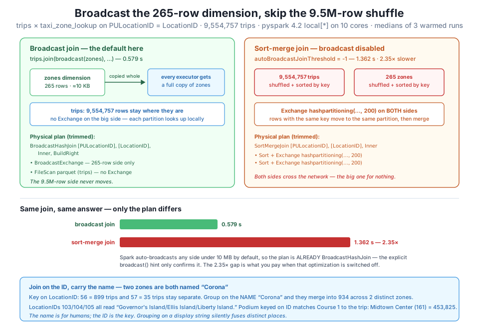
BroadcastHashJoin with no Exchange on the big side, 0.579 s. Disabling auto-broadcast forces a SortMergeJoin that shuffles both sides through Exchange hashpartitioning(…, 200), 1.362 s — 2.35× slower for the identical answer. Spark auto-broadcasts under 10 MB, so the default plan is already broadcast; the hint only confirms it. Footer: key on LocationID (Corona 56 = 899, 57 = 35), never the name, which fuses them into 934.The busiest zones, finally with names
Keyed on LocationID and carrying the name for display, the quarter’s podium reads Midtown Center (161) 453,825 · Upper East Side South (237) 439,138 · JFK Airport (132) 429,745 · Upper East Side North (236) 416,508 · Midtown East (162) 336,460 — Course 1’s ground truth, to the trip, now legible. Group that same query on Zone instead and Midtown Center would be fine, but every “Corona” trip in the borough would land in one invented row. The join gave the numbers names; keying on the ID kept the names honest.
Exercise 1 — Which zones had no pickups? You proved 0 trips are orphaned from the dimension. Ask the mirror-image question: which of the 265 zones served as a pickup for zero trips this quarter? Run a left_anti join with zones on the left and the trips’ distinct PULocationID on the right (zones.join(trips.select("PULocationID").distinct(), zones.LocationID == F.col("PULocationID"), "left_anti")), count the result, and list a few. Explain why this is a left_anti and not a left join.
Hint
There were 262 distinct pickup IDs among 265 zones, so expect a small number of never-used zones. left_anti is right because you want the zones with no match in the trips and you want none of the trips’ columns — just the unused dimension rows. A left join would instead keep all 265 zones and null the trip side, forcing you to filter for the nulls yourself; left_anti is that filter, done in one step and without widening the row.
Exercise 2 — Make Spark show you the shuffle. Take the plain trips.join(zones, ...) (no broadcast()), call .explain(), and confirm it’s a BroadcastHashJoin. Now set spark.conf.set("spark.sql.autoBroadcastJoinThreshold", -1), build the same join, and .explain() again. Identify the two Exchange hashpartitioning(..., 200) nodes and the join type that replaced the broadcast. Restore the default (10 * 1024 * 1024) and confirm the broadcast returns. Write one sentence on what the 200 means and why it’s wasteful for a 265-row dimension.
Hint
The 200 is spark.sql.shuffle.partitions, Spark’s cluster-scale default number of post-shuffle partitions — the same knob Lesson 1’s exercises turned. Shuffling a 265-row table into 200 partitions means most partitions get one row or none, pure scheduling overhead. That is exactly the waste the broadcast join skips: with BroadcastHashJoin there is no post-shuffle stage on either side, so spark.sql.shuffle.partitions never enters the picture for this join. Adaptive Query Execution coalesces some of the empty partitions, which is why the measured gap is smaller than the 200-vs-1 ratio suggests.
Exercise 3 — Catch a collision in the act. Build the full named podium two ways: once grouped on PULocationID (carrying Zone for display) and once grouped on Zone alone, each counting trips and ordered descending. Join or compare the two rankings and find every Zone name whose by-name count exceeds the largest single-ID count under it — those are the fused names. Confirm “Corona” is among them (934 by name vs 899 for its biggest ID) and report any others you find.
Hint
The cleanest detector is countDistinct("PULocationID") inside a groupBy("Zone") — any Zone with a distinct-ID count above 1 is a collision. “Corona” (2 IDs) and “Governor’s Island/Ellis Island/Liberty Island” (3 IDs) are the ones in this dimension. The by-name total for Corona is 934 = 899 + 35; the fact that no single number in the by-name ranking is wrong is precisely what makes the trap dangerous — the merged row looks like a perfectly ordinary result.
You gave CityFlow’s numbers their names. Joining the quarter’s 9,554,757 trips to the 265-row taxi_zone_lookup on PULocationID == LocationID attached a borough and zone name to every trip; a left_anti join proved zero trips were orphaned (inner and left both returned 9,554,757), while surfacing that the dimension’s own junk codes — 264 (Unknown, null Zone, 31,588 trips) and 265 (Outside of NYC, 5,172 trips) — match the join but carry no real name, a different failure than a missing key and one you check separately. The broadcast join was the performance heart: because the dimension is ~10 KB, Spark auto-broadcasts it, so the default plan is already a BroadcastHashJoin with no Exchange on the 9.5 million-row side; disabling auto-broadcast forces a SortMergeJoin that shuffles both tables through Exchange hashpartitioning(..., 200) and runs 2.35x slower (1.362 s vs 0.579 s) on this run for the identical answer — the plan, not the fickle ratio, is the durable proof, and the explicit broadcast() hint mostly confirms what the optimizer already chose. The named borough rollup summed to $256,692,373.14 to the cent and the podium matched Course 1 to the trip (Midtown Center 453,825). And the key-on-ID trap: LocationID 56 and 57 are both “Corona” (899 and 35 trips), so grouping on the name fuses two distinct zones into one 934-trip row — names are labels, IDs are keys. Finally, self-joining the dimension for pickup and drop-off names produced an AMBIGUOUS_REFERENCE error that aliases (pickup, dropoff) resolve cleanly.
broadcast(df) forces it, BroadcastHashJoin with no Exchange on the big side confirms it, and Spark auto-broadcasts anything under spark.sql.autoBroadcastJoinThreshold (10 MB default).spark.sql.shuffle.partitions (200) and sorted before merging; correct for big-to-big, wasteful for big-to-tiny (2.35x slower here).LocationID; the Zone name is a non-unique display label, so grouping on it silently merges distinct zones (Corona 56 + 57 → one 934-trip row).AMBIGUOUS_REFERENCE; df.alias("x") plus qualified F.col("x.column") references make every column unambiguous.A dimension join is the most common operation in a data warehouse, and it hides two failure modes that both pass silently. The performance one — shuffling a billion-row fact table to meet a lookup that fits in memory — is invisible until the job that should take seconds takes an hour; you now read it straight off the physical plan (Exchange on the big side or not) and know the fix is a broadcast Spark usually applies for you, but that you can force when its size estimate is wrong. The correctness one is worse because the output looks fine: group your revenue report on a zone name and two real Coronas become one imaginary place, with no error, no null, no warning — just a number that’s the sum of two things that were never the same thing. CityFlow’s operations team will read these reports by name, so the discipline that keeps the join honest — key on the ID, carry the label, left_anti before you trust, alias before you self-join — is not pedantry; it’s the difference between a report someone can act on and a report that quietly lies. Every aggregation in the rest of this module rests on this join being both fast and true.
You can now attach a dimension to a fact table correctly and quickly: choose the join type from the question, prove there are no orphans with left_anti, let Spark broadcast the small side (or force it when you must), and key on the stable ID while carrying the name only for display. What you did to Borough — group the joined trips and sum revenue — was a preview of the operation the next lesson makes its whole subject. Lesson 4, GroupBy & Aggregation, takes the groupBy().agg() you leaned on here and opens it fully: multiple aggregations at once, count and sum and avg and countDistinct side by side, aggregating several columns, sorting and naming the results, and a first honest look at the shuffle a wide aggregation forces. You’ll rebuild the per-zone and per-zone-per-hour numbers this course keeps cross-checking, and you’ll do it keying on LocationID — because after this lesson, you know exactly what grouping on the name would cost.
Keep DATATWEETS free. Help fund practical data, AI, and engineering lessons for learners worldwide.
