Title here
Summary here
Every lesson in this module has been sharpening one column at a time. Lesson 1 built derived columns — a pickup hour out of a timestamp, a fare-per-mile out of two numbers. Lesson 2 cleaned the real taxi dirt and, crucially, kept the negative-amount fare reversals because dropping them would corrupt revenue by hundreds of thousands of dollars a month. Lesson 3 attached borough and zone names by joining on LocationID, never on the name, because two different zones both answer to “Corona.” You now have clean, labelled, per-trip rows. What you do not yet have is the move that turns 9.5 million rows into an answer a human can read: collapsing them into one row per group.
That move is groupBy().agg(), and it is the busiest verb in a data engineer’s day. This lesson makes you fluent in it on CityFlow’s real quarter. You’ll compute a rich per-zone summary — trips, revenue, average fare, average distance, distinct active hours — in a single pass, and watch the answer land exactly on Course 1’s verified podium (Midtown Center 453,825 trips, JFK 429,745). You’ll take the quarter’s entire revenue, $256,692,373.14, with a keyless one-liner that matches Course 1 to the cent. You’ll group by two keys at once to reach the report’s 240,917 zone-hour buckets. And you’ll read explain() to see the reason groupBy scales at all: Spark aggregates twice — once on the map side to shrink each partition, then once more after a small shuffle — so the network moves roughly 2,620 partial rows instead of 9.5 million. The full zone-hour report is Lesson 5’s job; here you install every mechanic it will assemble.
By the end of this lesson, you will be able to:
groupBy().agg() pass with F.count, F.sum, F.avg, F.min, F.max, F.stddev, and F.countDistinct, each .alias()-nameddf.agg() and cross-check them against Course 1’s ground truth to the centexplain() and recognize map-side partial aggregation (partial_sum, partial_count) as the reason a wide groupBy shuffle stays tinypivot, and judge honestly when its second pass is worth paying forYou’ll need pyspark (JDK 17 or 21 — see the course setup), pyspark.sql.functions, the three taxi-quarter Parquet files, and taxi_zone_lookup.csv.
One session for the whole lesson. Read the quarter, apply Lesson 2’s report window (2024-01-01 ≤ pickup < 2024-04-01, which quarantines the 21 stray-stamped trips), and derive the hourly bucket with Lesson 1’s date_trunc so it’s ready when we need it. Everything downstream groups this one trips DataFrame.
import warnings
warnings.filterwarnings("ignore")
from pyspark.sql import SparkSession
import pyspark.sql.functions as F

spark = (SparkSession.builder
         .appName("cityflow")
         .master("local[*]")
         .config("spark.ui.showConsoleProgress", "false")
         .getOrCreate())
spark.sparkContext.setLogLevel("ERROR")

QUARTER = ["yellow_tripdata_2024-01.parquet",
           "yellow_tripdata_2024-02.parquet",
           "yellow_tripdata_2024-03.parquet"]
quarter = spark.read.parquet(*QUARTER)
trips = (quarter
    .filter((F.col("tpep_pickup_datetime") >= "2024-01-01") &
            (F.col("tpep_pickup_datetime") < "2024-04-01"))
    .withColumn("pickup_hour", F.date_trunc("hour", "tpep_pickup_datetime")))
print("quarter partitions:", trips.rdd.getNumPartitions())
quarter partitions: 10Ten partitions, exactly as Module 2 established for the three-file quarter — a number that will matter the moment we look at the physical plan, because the first stage of every aggregation below runs one task per partition. Nothing has scanned yet; filter, withColumn, and date_trunc are all lazy, so this printed instantly and the real work waits for the first action.
Here is the shape you will type more than any other in this course. groupBy(key) returns a grouped object that does nothing on its own; .agg(...) attaches the aggregate expressions and returns a new DataFrame with one row per group. Each aggregate is an expression from pyspark.sql.functions, and each gets an .alias() so the output column has a name you chose instead of sum(total_amount). The decisive property: all of these are computed in a single pass over the data. Asking for five aggregates costs one scan, not five.
by_zone = trips.groupBy("PULocationID").agg(
    F.count("*").alias("trips"),
    F.round(F.sum("total_amount") / 1e6, 2).alias("revenue_musd"),
    F.round(F.avg("fare_amount"), 2).alias("avg_fare"),
    F.round(F.avg("trip_distance"), 2).alias("avg_dist"),
    F.countDistinct("pickup_hour").alias("distinct_hours"))

lookup = spark.read.option("header", True).csv("taxi_zone_lookup.csv")
named = (by_zone.join(F.broadcast(lookup),
                      by_zone.PULocationID == lookup.LocationID, "left")
                .select("Zone", "Borough", "trips", "revenue_musd",
                        "avg_fare", "avg_dist", "distinct_hours"))
named.orderBy(F.desc("trips")).show(5, truncate=False)
+---------------------+---------+------+------------+--------+--------+--------------+
|Zone |Borough |trips |revenue_musd|avg_fare|avg_dist|distinct_hours|
+---------------------+---------+------+------------+--------+--------+--------------+
|Midtown Center |Manhattan|453825|10.81 |15.55 |2.53 |2179 |
|Upper East Side South|Manhattan|439138|8.69 |12.49 |1.85 |2175 |
|JFK Airport |Queens |429745|33.14 |59.67 |15.59 |2183 |
|Upper East Side North|Manhattan|416508|8.48 |13.05 |2.43 |2150 |
|Midtown East |Manhattan|336460|7.83 |15.14 |2.56 |2180 |
+---------------------+---------+------+------------+--------+--------+--------------+
only showing top 5 rowsFive aggregates, one scan, and the answer is Course 1’s verified quarter podium to the trip: Midtown Center 453,825, Upper East Side South 439,138, JFK 429,745, Upper East Side North 416,508, Midtown East 336,460. Same data, same window, new engine, same truth. Read across a row and the aggregate tells a story a raw count cannot: JFK moves fewer trips than Midtown Center but bills $33.14M against Midtown’s $10.81M, because its $59.67 average fare (the flat airport rate over a 15.59-mile average haul) dwarfs Midtown’s $15.55 over 2.53 miles. That is the whole point of aggregation — a shape you can reason about instead of nine million you cannot.
Two details worth naming. I divided the revenue sum by 1e6 and rounded, so the column reads in millions of dollars; without it, show() prints a double like 1.081437978E7 in scientific notation, which is correct but hard to read (the exact-to-the-cent total is coming in a moment from a keyless aggregate). And I attached the borough and zone names with Lesson 3’s broadcast join on LocationID — the 265-row lookup is tiny, so Spark ships it to every task and skips a shuffle. Group first on the ID, label second; never group on the name.
The last column, distinct_hours, is the one to sit with. F.countDistinct("pickup_hour") counts how many distinct hourly buckets each zone saw at least one pickup in. The quarter spans 91 days, so the ceiling is $91 \times 24 = 2184$ buckets — and JFK, at 2183, missed exactly one hour in three months. Hold onto that number; it is a hidden bridge to the zone-hour report, and we’ll spend it shortly.
avg tells you the middle; it hides the shape. Swap in F.min, F.max, and F.stddev — same one-pass grammar, same .alias() discipline — and the reversals Lesson 2 fought to keep come into view.
spread = trips.groupBy("PULocationID").agg(
    F.count("*").alias("trips"),
    F.round(F.min("fare_amount"), 2).alias("min_fare"),
    F.round(F.avg("fare_amount"), 2).alias("avg_fare"),
    F.round(F.max("fare_amount"), 2).alias("max_fare"),
    F.round(F.stddev("fare_amount"), 2).alias("sd_fare"))
spread.orderBy(F.desc("trips")).show(5, truncate=False)
+------------+------+--------+--------+--------+-------+
|PULocationID|trips |min_fare|avg_fare|max_fare|sd_fare|
+------------+------+--------+--------+--------+-------+
|161 |453825|-367.7 |15.55 |761.1 |13.34 |
|237 |439138|-187.0 |12.49 |306.8 |9.31 |
|132 |429745|-739.4 |59.67 |912.3 |33.07 |
|236 |416508|-116.8 |13.05 |288.6 |9.47 |
|162 |336460|-484.6 |15.14 |484.6 |12.44 |
+------------+------+--------+--------+--------+-------+
only showing top 5 rowsEvery min_fare is negative — Midtown Center’s floor is -367.70, JFK’s -739.40. Those are the fare reversals Lesson 2 measured and deliberately did not drop: corrections booked as negative fares that a SUM cancels against their originals, which is exactly why revenue still totals correctly. If a well-meaning teammate had filtered fare_amount > 0 upstream, these floors would vanish and the quarter’s revenue would drift by the ±$0.8M/month Course 1 quantified. The aggregate makes the decision auditable: the reversals are right there in min_fare, not silently gone. Meanwhile JFK’s 33.07 standard deviation against a $59.67 mean confirms its bimodal fare structure (flat-rate airport runs plus metered exceptions), where Upper East Side South’s tight $9.31 spread around $12.49 says “short, predictable Manhattan hops.” Center and spread, computed together, cost the same single scan.
Sometimes you want no groups at all — one number for the whole dataset. Call .agg() directly on the DataFrame, with no groupBy in front, and Spark aggregates every row into a single output row. This is how you get the quarter’s headline revenue as a one-liner.
totals = trips.agg(
    F.round(F.sum("total_amount"), 2).alias("revenue"),
    F.count("*").alias("trips")).collect()[0]
print(f"quarter revenue: ${totals['revenue']:,.2f}")
print(f"quarter trips  : {totals['trips']:,}")
quarter revenue: $256,692,373.14
quarter trips : 9,554,757$256,692,373.14 across 9,554,757 trips — Course 1’s capstone number reproduced to the cent, on the same window, by a completely different engine. This is the cross-verification this course was built to demonstrate: the pandas-plus-multiprocessing pipeline from Course 1 and this one-line Spark aggregation are two roads to the identical penny. A keyless df.agg() is structurally a groupBy over a single, whole-dataset group — the same two-pass machinery you’re about to see in the plan, just with one group at the end. Reach for it whenever the question is “over everything, what is the total / count / max,” and reach for groupBy().agg() the moment the question gains a “per.”
groupBy takes as many keys as you hand it. Group by (PULocationID, pickup_hour) and each output row is one zone in one hour — precisely the grain the zone-hour report is defined on. The result’s row count is the number of distinct (zone, hour) combinations that actually occurred.
by_zone_hour = trips.groupBy("PULocationID", "pickup_hour").agg(
    F.count("*").alias("trips"),
    F.round(F.sum("total_amount"), 2).alias("revenue"))
print("zone-hour buckets:", by_zone_hour.count())
print("sum of distinct_hours:",
      by_zone.agg(F.sum("distinct_hours")).collect()[0][0])
zone-hour buckets: 240917
sum of distinct_hours: 240917240,917 — Course 1’s exact bucket count, reached here with nothing but a two-key groupBy. And the second line closes a loop from earlier: summing each zone’s distinct_hours (from the single-key aggregate) gives the same 240,917, because a zone’s count of active hourly buckets, summed across all 262 zones, is the number of (zone, hour) pairs. Two different groupings, one identity — a satisfying internal cross-check that the mechanics are sound. Adding a key multiplied the output from 262 rows to 240,917, but the code barely changed and it is still one pass. That is the entire skeleton of Lesson 5’s report: window, derive the hour, group by two keys, aggregate trips and revenue. This lesson proves each vertebra; the next assembles the spine and verifies all four numbers at once.
groupBy, not a window function
Everything here collapses rows: 9,554,757 trips become 262 zones or 240,917 buckets, and the per-trip detail is gone. When you instead need an aggregate alongside every original row — each trip labelled with its zone’s running total, or ranked within its hour — that is a window function (Window.partitionBy(…) with F.sum().over(…)), a different tool that keeps the rows and adds a column. It’s a later topic; for now, if the question ends in “per group, one number,” groupBy().agg() is the answer.
A groupBy is a wide transformation — the vocabulary from Module 2’s DAG lesson — because a zone’s rows start scattered across all 10 partitions and must be regrouped before they can be summed. Regrouping means a shuffle, and a shuffle is the expensive thing on a real cluster. So the natural worry is: does grouping 9.5 million rows mean shoving 9.5 million rows across the network? Read the plan and see.
trips.groupBy("PULocationID").agg(
    F.sum("total_amount").alias("revenue"),
    F.count("*").alias("trips")).explain()
== Physical Plan ==
AdaptiveSparkPlan isFinalPlan=false
+- HashAggregate(keys=[PULocationID#7], functions=[sum(total_amount#16), count(1)])
+- Exchange hashpartitioning(PULocationID#7, 200), ENSURE_REQUIREMENTS, [plan_id=634]
+- HashAggregate(keys=[PULocationID#7], functions=[partial_sum(total_amount#16), partial_count(1)])
+- Project [PULocationID#7, total_amount#16]
+- Filter ((isnotnull(tpep_pickup_datetime#1) AND (tpep_pickup_datetime#1 >= 2024-01-01 00:00:00)) AND (tpep_pickup_datetime#1 < 2024-04-01 00:00:00))
+- FileScan parquet [tpep_pickup_datetime#1,PULocationID#7,total_amount#16] ...(The FileScan line’s path and pushed-filter detail are trimmed for width.) Read it bottom-up and the answer is unmistakable: there are two HashAggregate operators with the single Exchange between them. The lower one runs functions named partial_sum and partial_count — this is map-side partial aggregation, and it happens before the shuffle, independently on each of the 10 partitions. Each task collapses its slice down to at most one partial row per zone it saw — at most 262 rows — so what crosses the Exchange hashpartitioning is roughly $10 \times 262 \approx 2{,}620$ partial rows, not 9,554,757. The upper HashAggregate then does the reduce-side finish: it sums the partial sums and counts the partial counts into the final 262 zone totals. Two phases, one written groupBy.
This is the whole reason groupBy scales, and it is why the Module 2 lesson measured a “combine before you move” trick with a tiny shuffle-write for millions of input rows. sum and count are cleanly separable — a sum of partial sums is the true sum — so Spark can pre-aggregate. (Not every aggregate splits so neatly: countDistinct must reconcile which values it has already seen across partitions, so it cannot fully collapse map-side and is the pricier one in the row above — reach for it deliberately, not by reflex.) What that shuffle actually costs — the sort, the disk spill, the network — is Module 5’s entire subject; here the honest one-sentence version is that map-side pre-aggregation shrinks the bill by orders of magnitude before Module 5 ever tallies it. And note isFinalPlan=false: as Module 2 showed, adaptive query execution will re-plan at runtime, coalescing that 200-way shuffle down to a single finishing task because 2,620 rows need nothing more.
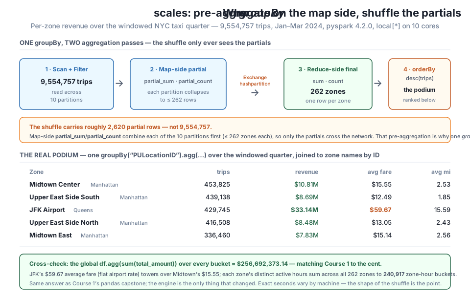
groupBy(“PULocationID”).agg(…) over 9,554,757 windowed trips, read from explain(). Spark aggregates twice: a map-side partial_sum/partial_count collapses each of the 10 partitions to ≤ 262 rows, so the Exchange moves roughly 2,620 partial rows instead of 9.5 million — then a reduce-side HashAggregate finishes the 262 zones. The podium matches Course 1 to the trip (Midtown Center 453,825 · JFK 429,745 at a $59.67 average fare) and the keyless total, $256,692,373.14, matches to the cent.One more plan fact you already own: had we ended with .orderBy(F.desc("trips")) — as the podium display did — the plan would carry a second Exchange, a rangepartitioning, plus a hidden sampling job to choose balanced sort ranges. Module 2 measured exactly that. It’s cheap here because only 262 rows sort, but it is a real second shuffle; sort the aggregated result, never the raw trips.
pivot turns distinct values of a column into columns of their own. Slot it between groupBy and agg: group by the row key, pivot the column key, aggregate the cell. Here, borough down the side and time-of-day across the top, counting trips per cell. Deriving a coarse daypart first keeps the pivot small, and passing the explicit value list avoids an extra scan Spark would otherwise spend discovering the distinct values.
by_borough = (trips.join(F.broadcast(lookup),
                         trips.PULocationID == lookup.LocationID, "left")
    .withColumn("hr", F.hour("tpep_pickup_datetime"))
    .withColumn("daypart",
        F.when(F.col("hr") < 6, "Night")
         .when(F.col("hr") < 12, "Morning")
         .when(F.col("hr") < 18, "Afternoon")
         .otherwise("Evening")))
pivoted = (by_borough.groupBy("Borough")
    .pivot("daypart", ["Night", "Morning", "Afternoon", "Evening"])
    .agg(F.count(F.lit(1))))
pivoted.orderBy(F.desc("Afternoon")).show(truncate=False)
+-------------+------+-------+---------+-------+
|Borough |Night |Morning|Afternoon|Evening|
+-------------+------+-------+---------+-------+
|Manhattan |690070|1848145|3073332 |2945202|
|Queens |58700 |164185 |303887 |311110 |
|Brooklyn |14950 |33240 |25240 |23789 |
|Unknown |2797 |7420 |11323 |10048 |
|Bronx |2746 |11521 |7394 |3298 |
|NULL |1125 |1021 |1551 |1475 |
|EWR |74 |172 |526 |182 |
|Staten Island|58 |50 |72 |54 |
+-------------+------+-------+---------+-------+The cross-tab reads at a glance: Manhattan’s afternoon peak of 3,073,332 trips is the city’s engine, while Queens is the one borough that pivots to a heavier evening (311,110) than afternoon — the shape of JFK’s late-arrival traffic. Two honest footnotes. The NULL row is pickups whose LocationID has no match in the lookup, and the Unknown row is the lookup’s own placeholder zones — the key-on-ID reality Lesson 3 flagged, surfacing here as a small unlabelled tail you’d quarantine or investigate, never silently drop. And pivot is genuinely a second aggregation pass layered on the group; supplying the value list keeps it to one extra scan rather than two, but on a wide, high-cardinality key it can grow expensive fast. Use it for small, known categoricals like these four dayparts; for a hundred columns, group long and reshape elsewhere.
Prefer built-in aggregates over UDFs
Every aggregate in this lesson — sum, count, stddev, countDistinct — is a built-in from pyspark.sql.functions, which is why Catalyst could split each into the map-side/reduce-side phases you saw in the plan. A Python UDF is opaque to that optimizer: it cannot pre-aggregate what it cannot see inside, so the whole group would cross the shuffle uncombined. Module 4 measures that cost directly; the habit to build now is to check the functions module first and only write a UDF when nothing there fits.
Close the session — it’s the last block, so the tracker and the UI at localhost:4040 go down with it.
spark.stop()
print("session closed")
session closedExercise 1 — A payment-type profile in one pass. Group the windowed trips by payment_type and, in a single .agg(), compute the trip count, the summed total_amount (in millions), the average tip_amount, and the maximum tip_amount — each .alias()-named. Sort by trip count descending and read the result: which payment type tips, which structurally cannot, and what the largest single tip in the quarter was.
Hint
The grammar is identical to the per-zone aggregate: trips.groupBy(“payment_type”).agg(F.count("*").alias(“trips”), F.round(F.sum(“total_amount”)/1e6, 2).alias(“revenue_musd”), F.round(F.avg(“tip_amount”),2).alias(“avg_tip”), F.round(F.max(“tip_amount”),2).alias(“max_tip”)). Payment type 1 is card and 2 is cash; TLC records cash tips as 0, so cash’s avg_tip being ~0 is a data-collection fact, not a stinginess fact — exactly the kind of caveat an aggregate makes visible.
Exercise 2 — Confirm the two-key identity. You saw that sum(distinct_hours) over zones equals the 240,917 zone-hour buckets. Now verify the revenue is conserved the same way: build by_zone_hour (group by PULocationID, pickup_hour, summing total_amount), then take by_zone_hour.agg(F.sum("revenue")) and confirm it lands on $256,692,373.14 — the same grand total the keyless df.agg() produced. Explain in one sentence why regrouping into 240,917 finer buckets and then summing must return the identical total.
Hint
A sum is associative: partitioning 9,554,757 trips into 262 zones, or into 240,917 zone-hours, or into one whole-dataset group, only changes how the additions are bracketed, never the result. If your finer-grained total is off by a rounding cent, sum the unrounded column and round once at the end — round each bucket and the pennies accumulate.
Exercise 3 — Watch the plan lose its map-side phase. Run explain() on two aggregations of trips grouped by PULocationID: first F.sum("total_amount"), then F.countDistinct("pickup_hour"). Compare the two physical plans. Which one shows partial_sum beneath the Exchange, and which one cannot fully pre-aggregate before the shuffle? Write one sentence connecting what you see to why countDistinct is the more expensive aggregate in this lesson’s per-zone table.
Hint
Look for the paired HashAggregate operators with partial_ functions in the lower one — the sum plan has them. A distinct count must know which pickup_hour values it has already counted across every partition, so it can’t collapse each partition to one number independently; expect its plan to carry the raw distinct keys further before the final reconciliation. Same groupBy syntax, very different physics underneath — reading the plan is how you tell them apart before the cluster bills you.
groupBy().agg() is the verb that turns nine and a half million rows into an answer, and this lesson made it fluent on CityFlow’s real quarter. A single pass with F.count, F.sum, F.avg, F.min, F.max, F.stddev, and F.countDistinct — each .alias()-named — produced a per-zone profile that matched Course 1’s podium to the trip (Midtown Center 453,825, JFK 429,745 billing $33.14M at a $59.67 average fare) while the min_fare column kept Lesson 2’s negative reversals auditable instead of silently dropped. A keyless df.agg() returned the quarter’s entire revenue, $256,692,373.14 over 9,554,757 trips, matching Course 1 to the cent; adding a second key reached the report’s 240,917 zone-hour buckets, which equal the summed per-zone distinct_hours by a satisfying identity. And explain() revealed why a wide groupBy scales: two HashAggregate phases around one Exchange, the lower running partial_sum/partial_count so the shuffle carries roughly 2,620 partial rows instead of 9.5 million. pivot reshaped borough by daypart in a small, honest cross-tab, with the reminder that it is a second pass to spend deliberately. Every number here is Course 1’s, reproduced by a different engine — the cross-verification this course exists to demonstrate.
groupBy().agg() — the workhorse: a grouped object plus aggregate expressions returns one row per group, computing every requested aggregate in a single pass. Alias each aggregate; group on stable IDs and label with a broadcast join afterward.df.agg() — aggregation with no groupBy, collapsing the whole dataset to one row (grand total, count, max). Structurally a single-group groupBy; the road to the cross-checkable $256,692,373.14.groupBy(k1, k2) produces one row per distinct combination; the row count is the number of combinations that occurred (240,917 zone-hours), and coarser and finer groupings of a sum always reconcile.partial_sum/partial_count HashAggregate beneath the Exchange in explain(): each partition pre-combines before the shuffle, so ~2,620 partial rows move instead of millions. The reason groupBy scales — and the reason countDistinct, which can’t fully pre-combine, costs more.pivot — distinct values of a column become output columns, a cross-tab in one statement; a genuine second pass, cheap for small known categoricals (four dayparts) and expensive for wide keys.CityFlow’s entire reporting layer is groupBy().agg() — revenue per zone, trips per hour, tips per payment type are the daily questions, and the engineer who writes them fluently, aliases them cleanly, and cross-checks the totals is the one whose dashboards are trusted. But fluency without the plan underneath is fragile: the engineer who reads partial_sum in explain() knows why a per-zone aggregate over the whole city returns in seconds while a countDistinct over the same key drags, and can choose the cheaper aggregate before the cluster invoices the difference — the judgment Module 5 will price in full. Most of all, this lesson is the dress rehearsal. Every mechanic here — the window, the derived hour, the two-key group, the broadcast label-join, the reconciled total — is a part the next lesson bolts together into Course 1’s complete zone-hour report, rebuilt in idiomatic Spark and verified against all four ground-truth numbers at once. You now have every part; next you assemble the machine.
You have proven each mechanic in isolation, and they all landed on Course 1’s verified numbers: the podium to the trip, the revenue to the cent, the buckets to the unit. Lesson 5, Guided Project: The Zone-Hour Report, is where they stop being exercises and become a pipeline. You’ll read the three months, apply the window that keeps the reversals and quarantines the 21 strays, derive the pickup hour, group by (zone, hour) and aggregate trips and revenue, join the zone names on LocationID, and produce the finished report — then verify, in one run, all four of Course 1’s ground-truth figures simultaneously: 240,917 buckets, 9,554,757 trips kept, $256,692,373.14 in revenue, and the podium to the digit. It is the module’s payoff and Course 1’s capstone reproduced on a cluster-scale engine, delivered as a clean, reusable script with explicit acceptance criteria. Bring today’s groupBy().agg() fluency; you’ll use every line of it.
Keep DATATWEETS free. Help fund practical data, AI, and engineering lessons for learners worldwide.
