Title here
Summary here
Four lessons ago you could read a Spark DataFrame and print its schema. Since then you have learned to build columns with expressions (Lesson 1), to filter and clean the taxi data’s real dirt without deleting the reversals that a careless filter would corrupt (Lesson 2), to join the 265-row zone dimension with a broadcast that skips the shuffle (Lesson 3), and to group and aggregate per zone and per hour (Lesson 4). Every one of those was a piece. This lesson is where the pieces become a job.
The job is a familiar one, and that is the entire point. Course 1’s capstone built CityFlow’s per-zone, per-hour trip and revenue report with pandas, multiprocessing, and a SQLite warehouse — streaming three months of real taxi data through a 400 MB memory budget and cross-checking the result against a full-load baseline to the cent. That project left an answer key: 240,917 (zone, hour) buckets, 9,554,757 trips kept, 21 quarantined, and $256,692,373.14 of revenue, with a busiest-zone podium led by Midtown Center at 453,825 pickups. Now you rebuild that same report in idiomatic Spark — the DataFrame API you have spent the module learning — and hold the new engine to the old numbers. If Spark disagrees with any of them, the new code is wrong; the ground truth is not up for debate. By the end of this page a reusable script prints one page and passes 9 of 9 cross-checks against Course 1.
By the end of this project, you will be able to:
$256,692,373.14 to the centgroupBy().agg() and cross-check the bucket count and trip total to the digitLocationID, keeping the two distinct “Corona” zones separatemain(), explicit cross-checks, spark.stop() — and contrast its shape with Course 1’s pandas pipelineYou’ll need pyspark (with the Java 17/21 runtime from the course setup page); everything else is the Python standard library.
A guided project earns its name from its acceptance criteria — the checks that turn “the code ran” into “the report is right.” Before any Spark, here is what “done” means for the zone-hour report, and every one is a number Course 1 already established:
groupBy(zone, hour).agg(trips, revenue) → broadcast-join the zone names on LocationID.(zone, hour) buckets whose trip counts sum back to 9,554,757.total_amount inside the window prints as $256,692,373.14.main() that creates its session, prints one page of labelled cross-checks, and calls spark.stop().The data is New York City’s public-domain Yellow Taxi trip records, published by the NYC Taxi & Limousine Commission on its Trip Record Data page — the same three months Course 1 processed, plus the 265-row zone lookup:
https://d37ci6vzurychx.cloudfront.net/trip-data/yellow_tripdata_2024-01.parquet (2,964,624 rows)https://d37ci6vzurychx.cloudfront.net/trip-data/yellow_tripdata_2024-02.parquet (3,007,526 rows)https://d37ci6vzurychx.cloudfront.net/trip-data/yellow_tripdata_2024-03.parquet (3,582,628 rows)https://datatweets.com/datasets/nyc-taxi/taxi_zone_lookup.csv (265 zones)A real pipeline downloads once and reads local copies, so every runnable block below uses the bare filenames:
# gate: skip
# Fetch once; every block afterwards reads the local cached copies by name.
import urllib.request
for m in ("01", "02", "03"):
    urllib.request.urlretrieve(
        f"https://d37ci6vzurychx.cloudfront.net/trip-data/yellow_tripdata_2024-{m}.parquet",
        f"yellow_tripdata_2024-{m}.parquet")
urllib.request.urlretrieve(
    "https://datatweets.com/datasets/nyc-taxi/taxi_zone_lookup.csv",
"taxi_zone_lookup.csv")Like every Spark job in this course, the report opens one SparkSession, uses it for everything, and stops it at the very end. This is the standard builder from Module 1 — local[*] for all ten cores, progress bars off so the pasted output stays clean, log level at ERROR so warnings don’t bury results.
import warnings; warnings.filterwarnings("ignore")
import time
from pyspark.sql import SparkSession
from pyspark.sql import functions as F
from pyspark.sql.functions import broadcast

t0 = time.perf_counter()
spark = (SparkSession.builder
         .appName("cityflow-zone-hour")
         .master("local[*]")
         .config("spark.ui.showConsoleProgress", "false")
         .getOrCreate())
spark.sparkContext.setLogLevel("ERROR")
print(f"SparkSession up in {time.perf_counter() - t0:.1f} s "
      f"(Spark {spark.version}, master {spark.sparkContext.master})")
SparkSession up in 5.1 s (Spark 4.2.0, master local[*])Five seconds of fixed cost before a single row moves — Module 1’s tax, paid once, up front. For the rest of the job the engine is warm, and the Spark UI is live at localhost:4040 if you want to watch each job land as the report builds.
Course 1 spent a whole module learning to stream these three files one row group at a time, because pandas would materialize them at 8.4x their disk size. Spark’s answer is one multi-path read.parquet call and a single count() to confirm the quarter arrived whole.
PATHS = [f"yellow_tripdata_2024-{m:02d}.parquet" for m in (1, 2, 3)]
trips = spark.read.parquet(*PATHS)
total = trips.count()
print(f"quarter rows read: {total:,}   (expected 9,554,778)")
quarter rows read: 9,554,778 (expected 9,554,778)9,554,778 — the quarter, exactly as Course 1 and Module 1’s guided project both counted it. That number is the raw input; every acceptance criterion below is about what survives the window, so keep it as the denominator the quarantine count subtracts from.
This is the step where careless code silently corrupts the answer, and where Lesson 2’s discipline pays off. The report is defined over one window — — so the filter is a where on the pickup timestamp. Because the column is timestamp_ntz, Spark casts the string literals to the column’s type for you, and the whole class of microsecond-versus-nanosecond unit bugs Course 1 fought disappears.
LO, HI = "2024-01-01", "2024-04-01"
in_window = trips.where((F.col("tpep_pickup_datetime") >= LO) &
                        (F.col("tpep_pickup_datetime") < HI))

kept = in_window.count()
print(f"kept       : {kept:,}   (expected 9,554,757)")
print(f"quarantined: {total - kept:>9}   (expected 21)")
kept : 9,554,757 (expected 9,554,757)
quarantined: 21 (expected 21)Criterion 2’s first half, met: 9,554,757 kept, 21 quarantined — the 2002/2009 relics and late-December stamps that fall outside the quarter, gone from the report but never deleted from trips. Now the half that separates a right pipeline from a fast-and-wrong one. The window filter is a time filter, not a sign filter: it keeps every negative-total fare reversal that falls inside the quarter. Watch what those reversals are worth, and what deleting them would cost.
acct = in_window.agg(
    F.count(F.when(F.col("total_amount") < 0, 1)).alias("reversals"),
    F.sum("total_amount").alias("revenue_kept"),
    F.sum(F.when(F.col("total_amount") >= 0, F.col("total_amount"))).alias("revenue_dropped"),
).collect()[0]

inflation = acct["revenue_dropped"] - acct["revenue_kept"]
print(f"in-window reversals kept : {acct['reversals']:,}")
print(f"revenue, reversals kept  : ${acct['revenue_kept']:,.2f}")
print(f"revenue, negatives dropped: ${acct['revenue_dropped']:,.2f}")
print(f"what dropping them inflates: ${inflation:,.2f}")
in-window reversals kept : 115,894
revenue, reversals kept : $256,692,373.14
revenue, negatives dropped: $259,679,181.90
what dropping them inflates: $2,986,808.76115,894 reversals ride inside the window, and they are load-bearing. A reversal is a +X charge and its −X void; kept together they cancel inside SUM. Drop the negative half with a where(total_amount >= 0) — the “clean the data” instinct — and the voided charges silently re-enter, inflating the quarter’s revenue by $2,986,808.76, nearly three million dollars of error on a number this job is being held to at the cent. The correct policy is Course 1’s, now expressed in Spark: count the reversals, keep them, let the sum cancel them. Everything downstream aggregates in_window, negatives and all.
The report’s grain is (zone, hour), so every trip needs an hour label. Lesson 1’s warning applies: the label you want is not the hour-of-day (0–23) — that would collapse the whole quarter into 24 buckets per zone. It is the pickup timestamp truncated to the hour, so each distinct calendar hour is its own bucket. F.date_trunc("hour", ...) does exactly that, and like every column expression it is lazy — it adds a node to the plan, nothing computes yet.
hourly = in_window.withColumn(
    "pickup_hour", F.date_trunc("hour", F.col("tpep_pickup_datetime")))

(hourly.select("tpep_pickup_datetime", "PULocationID", "pickup_hour", "total_amount")
 .show(5, truncate=False))
+--------------------+------------+-------------------+------------+
|tpep_pickup_datetime|PULocationID|pickup_hour |total_amount|
+--------------------+------------+-------------------+------------+
|2024-01-01 00:57:55 |186 |2024-01-01 00:00:00|22.7 |
|2024-01-01 00:03:00 |140 |2024-01-01 00:00:00|18.75 |
|2024-01-01 00:17:06 |236 |2024-01-01 00:00:00|31.3 |
|2024-01-01 00:36:38 |79 |2024-01-01 00:00:00|17.0 |
|2024-01-01 00:46:51 |211 |2024-01-01 00:00:00|16.1 |pickup_hour floors each timestamp to the top of its hour — 00:57:55 and 00:03:00 both become 2024-01-01 00:00:00, so they land in the same bucket for zone 186 versus 140. This is the same datetime64[h] bucketing Course 1 did with a NumPy cast, expressed as one Spark function. Truncating to the hour rather than extracting the hour-of-day is what makes the bucket count come out in the hundreds of thousands instead of two dozen — which the next step confirms against the ground truth.
groupBy(zone, hour) — the report’s coreNow the aggregation the whole report is built on. Group hourly by PULocationID and pickup_hour, and in one agg compute both measures: the trip count and the revenue sum. Because every later cross-check reads this result several times, cache it once — it is a small frame (240,917 rows), and caching means the 9.5-million-row scan behind it happens once instead of once per check.
report = (hourly.groupBy("PULocationID", "pickup_hour")
          .agg(F.count("*").alias("trips"),
               F.sum("total_amount").alias("revenue")))
report.cache()

n_buckets = report.count()
agg = report.agg(F.sum("trips").alias("trips"),
                 F.sum("revenue").alias("revenue")).collect()[0]

print(f"(zone, hour) buckets: {n_buckets:,}   (expected 240,917)")
print(f"trips across buckets: {agg['trips']:,}   (expected 9,554,757)")
print(f"raw float64 revenue : {agg['revenue']!r}")
print(f"revenue             : ${agg['revenue']:,.2f}   (expected $256,692,373.14)")
(zone, hour) buckets: 240,917 (expected 240,917)
trips across buckets: 9,554,757 (expected 9,554,757)
raw float64 revenue : 256692373.13999972
revenue : $256,692,373.14 (expected $256,692,373.14)Three criteria in one output. 240,917 buckets — the exact shape Course 1’s streaming aggregator produced. The trip counts sum back to 9,554,757, so no trip was lost or double-counted in the shuffle. And the revenue rounds to $256,692,373.14 — but look at the raw value, because it is quietly instructive. Spark returned 256692373.13999972. Module 1’s guided project, summing the same column over the same window, returned 256692373.14026505. Course 1’s serial pandas total was a third value again. None of them are wrong: float64 addition is not associative, and grouping by (zone, hour) before summing the buckets changes the order in which nine and a half million doubles are added. The last few bits move; the answer, to the cent, does not. That agreement-after-rounding, cross-checked against an independent computation, is exactly what “revenue to the cent” honestly means.
The report aggregates on PULocationID — a number — because Lesson 3 established that the zone dimension’s names are not unique: two Queens zones are both called “Corona.” Names come last, joined on the ID for display only. The dimension is 265 rows, so this is the textbook case for a broadcast join: ship the tiny table to every executor and join in place, with no shuffle of the big side.
zones = (spark.read.option("header", True).option("inferSchema", True)
         .csv("taxi_zone_lookup.csv")
         .select("LocationID", "Borough", "Zone"))
print(f"zone dimension: {zones.count()} rows")

named = report.join(broadcast(zones),
                    F.col("PULocationID") == F.col("LocationID"), "left")
named.explain()
zone dimension: 265 rows
== Physical Plan ==
AdaptiveSparkPlan isFinalPlan=false
+- BroadcastHashJoin [PULocationID#7], [LocationID#62], LeftOuter, BuildRight, false, false
:- HashAggregate(keys=[PULocationID#7, pickup_hour#20], functions=[count(1), sum(total_amount#16)])
: +- Exchange hashpartitioning(PULocationID#7, pickup_hour#20, 200), ENSURE_REQUIREMENTS, ...
: +- HashAggregate(keys=[PULocationID#7, pickup_hour#20], functions=[partial_count(1), partial_sum(total_amount#16)])
: +- Project [PULocationID#7, total_amount#16, date_trunc(hour, cast(tpep_pickup_datetime#1 as timestamp), Some(Asia/Tehran)) AS pickup_hour#20]
: +- Filter ((isnotnull(tpep_pickup_datetime#1) AND (tpep_pickup_datetime#1 >= 2024-01-01 00:00:00)) AND (tpep_pickup_datetime#1 < 2024-04-01 00:00:00))
: +- FileScan parquet [tpep_pickup_datetime#1,PULocationID#7,total_amount#16] ... ReadSchema: struct<tpep_pickup_datetime:timestamp_ntz,PULocationID:int,total_amount:double>
+- BroadcastExchange HashedRelationBroadcastMode(...), [plan_id=50]
+- Filter isnotnull(LocationID#62)
+- FileScan csv [LocationID#62,Borough#63,Zone#64] ...(The FileScan paths are trimmed for width.) The plan is worth reading, because it shows the join costing almost nothing. The top node is a BroadcastHashJoin, not the shuffle-based SortMergeJoin a naive join would pick. The only Exchange in the tree belongs to the groupBy shuffle — the aggregation’s cost, which we always pay — and there is no second shuffle for the join: the 265-row dimension goes into a BroadcastExchange and rides along to wherever the aggregated rows already are. One detail carried over from Module 1: date_trunc prints Some(Asia/Tehran) — the session’s time zone, which Spark records inside the expression. It is harmless here (the timestamps are wall-clock timestamp_ntz and the window literals are compared in the same zone), and it is a good reminder that a plan shows you the engine’s real assumptions, not just your code.
The report now carries names. Roll the hourly buckets up to per-zone totals, sort by trips, and check the top five against Course 1’s podium — not just the ranking, but the exact counts.
by_zone = (named.groupBy("PULocationID", "Zone", "Borough")
           .agg(F.sum("trips").alias("trips"),
                F.sum("revenue").alias("revenue"))
           .orderBy(F.desc("trips")))

EXPECTED = [("Midtown Center", 453_825), ("Upper East Side South", 439_138),
            ("JFK Airport", 429_745), ("Upper East Side North", 416_508),
            ("Midtown East", 336_460)]

print("  rank  zone                    borough        trips     revenue      check")
for i, (r, (ez, en)) in enumerate(zip(by_zone.limit(5).collect(), EXPECTED), 1):
    status = "OK" if (r["Zone"], r["trips"]) == (ez, en) else "MISMATCH"
    print(f"  {i}.    {r['Zone']:<22} {r['Borough']:<10} {r['trips']:>8,}  "
          f"${r['revenue']:>14,.2f}   {status}")
rank zone borough trips revenue check
1. Midtown Center Manhattan 453,825 $ 10,814,379.78 OK
2. Upper East Side South Manhattan 439,138 $ 8,694,610.47 OK
3. JFK Airport Queens 429,745 $ 33,137,512.96 OK
4. Upper East Side North Manhattan 416,508 $ 8,477,163.42 OK
5. Midtown East Manhattan 336,460 $ 7,829,595.20 OKFive zones, five exact matches — the same ranking and the same trip counts Course 1’s pipeline produced, down to the last digit, from an engine that partitioned the work across ten cores in whatever order the scheduler chose. The revenue column carries its own story: JFK is third by trips but first by dollars — $33.1M against Midtown Center’s $10.8M — because airport runs are long. Now the trap this whole discipline was built to avoid. Are the two Coronas still distinct?
coronas = (by_zone.where(F.col("Zone") == "Corona")
           .select("PULocationID", "Borough", "Zone", "trips")
           .orderBy("PULocationID").collect())
for r in coronas:
    print(f"  LocationID {r['PULocationID']} ({r['Borough']}): {r['trips']} trips")
LocationID 56 (Queens): 899 trips
LocationID 57 (Queens): 35 tripsTwo rows, kept separate: LocationID 56 with 899 trips and 57 with 35 — Course 1’s numbers exactly. Had the join keyed on Zone instead of the ID, these would have fused into one “Corona” with 934 trips and been wrong about both. Aggregating on the number and joining the name last is not a stylistic preference; it is the difference between a right report and a plausible one.
Every criterion has now been met interactively. Criterion 6 asks for the artifact CityFlow keeps — the file a teammate runs next Tuesday to get the same page. Each step above becomes a small function; zone_hour_report() is the pipeline itself, build_report() runs the cross-checks and renders one page, and main() owns the session lifecycle. Every [OK] is a live comparison against the GROUND dictionary — run it on the wrong files and the page fills with [MISMATCH].
report.unpersist()   # free the interactive cache; the script builds its own


def get_session():
    spark = (SparkSession.builder
             .appName("cityflow-zone-hour")
             .master("local[*]")
             .config("spark.ui.showConsoleProgress", "false")
             .getOrCreate())
    spark.sparkContext.setLogLevel("ERROR")
    return spark


MONTHS = ["2024-01", "2024-02", "2024-03"]
WINDOW = ("2024-01-01", "2024-04-01")
ZONE_LOOKUP = "taxi_zone_lookup.csv"
GROUND = {
    "buckets": 240_917, "trips_kept": 9_554_757, "quarantined": 21,
    "revenue": "256,692,373.14",
    "podium": [("Midtown Center", 453_825), ("Upper East Side South", 439_138),
               ("JFK Airport", 429_745), ("Upper East Side North", 416_508),
               ("Midtown East", 336_460)],
}


def read_quarter(spark):
    """All three months in one multi-path read."""
    paths = [f"yellow_tripdata_{m}.parquet" for m in MONTHS]
    return spark.read.parquet(*paths)


def zone_hour_report(spark, trips):
    """The module's whole pipeline: window -> hour -> groupBy -> broadcast-join names."""
    lo, hi = WINDOW
    in_window = trips.where((F.col("tpep_pickup_datetime") >= lo) &
                            (F.col("tpep_pickup_datetime") < hi))
    hourly = in_window.withColumn(
        "pickup_hour", F.date_trunc("hour", F.col("tpep_pickup_datetime")))
    buckets = (hourly.groupBy("PULocationID", "pickup_hour")
               .agg(F.count("*").alias("trips"),
                    F.sum("total_amount").alias("revenue")))
    zones = (spark.read.option("header", True).option("inferSchema", True)
             .csv(ZONE_LOOKUP).select("LocationID", "Borough", "Zone"))
    return buckets.join(broadcast(zones),
                        F.col("PULocationID") == F.col("LocationID"), "left")


def build_report(spark):
    """Build the report, cross-check every headline against Course 1, render one page."""
    t0 = time.perf_counter()
    trips = read_quarter(spark)
    total = trips.count()
    report = zone_hour_report(spark, trips)
    report.cache()

    n_buckets = report.count()
    agg = report.agg(F.sum("trips").alias("t"),
                     F.sum("revenue").alias("r")).collect()[0]
    trips_kept, revenue = agg["t"], agg["r"]
    podium = (report.groupBy("PULocationID", "Zone", "Borough")
              .agg(F.sum("trips").alias("trips"), F.sum("revenue").alias("revenue"))
              .orderBy(F.desc("trips")).limit(5).collect())
    corona = {r["PULocationID"]: r["trips"] for r in
              (report.groupBy("PULocationID", "Zone").agg(F.sum("trips").alias("trips"))
               .where(F.col("Zone") == "Corona").collect())}
    report.unpersist()

    checks = []

    def ok(cond):
        checks.append(bool(cond))
        return "[OK]" if cond else "[MISMATCH]"

    rev_str = f"{revenue:,.2f}"
    W = 66
    lines = ["=" * W,
             " CITYFLOW -- THE ZONE-HOUR REPORT (2024 Q1, NYC yellow taxi)",
             f" engine: Spark {spark.version}, local[*] -- cityflow_zone_hour_report.py",
             "=" * W, "",
             " SHAPE OF THE REPORT",
             f"   (zone, hour) buckets   {n_buckets:>11,}   {ok(n_buckets == GROUND['buckets'])}",
             f"   trips kept             {trips_kept:>11,}   {ok(trips_kept == GROUND['trips_kept'])}",
             f"   quarantined (window)   {total - trips_kept:>11,}   {ok(total - trips_kept == GROUND['quarantined'])}",
             f"   total revenue          ${rev_str:>12}   {ok(rev_str == GROUND['revenue'])}",
             "",
             f" BUSIEST PICKUP ZONES ({WINDOW[0]} <= pickup < {WINDOW[1]})"]
    for i, (r, (ez, en)) in enumerate(zip(podium, GROUND["podium"]), 1):
        lines.append(f"   {i}. {r['Zone']:<22} {r['Borough']:<10} {r['trips']:>8,}  "
                     f"${r['revenue']:>14,.2f}   {ok((r['Zone'], r['trips']) == (ez, en))}")
    lines += ["      (names joined on LocationID -- two zones are both 'Corona':",
              f"       56 -> {corona.get(56)} trips, 57 -> {corona.get(57)} trips)",
              "",
              f" VERDICT: {sum(checks)} of {len(checks)} cross-checks vs Course 1 passed.",
              f" built in {time.perf_counter() - t0:.1f} s (warm session)",
              "=" * W]
    return "\n".join(lines), sum(checks) == len(checks)


def main():
    spark = get_session()
    page, passed = build_report(spark)
    print(page)
    spark.stop()
    return passed


main()
==================================================================
CITYFLOW -- THE ZONE-HOUR REPORT (2024 Q1, NYC yellow taxi)
engine: Spark 4.2.0, local[*] -- cityflow_zone_hour_report.py
==================================================================
SHAPE OF THE REPORT
(zone, hour) buckets 240,917 [OK]
trips kept 9,554,757 [OK]
quarantined (window) 21 [OK]
total revenue $256,692,373.14 [OK]
BUSIEST PICKUP ZONES (2024-01-01 <= pickup < 2024-04-01)
1. Midtown Center Manhattan 453,825 $ 10,814,379.78 [OK]
2. Upper East Side South Manhattan 439,138 $ 8,694,610.47 [OK]
3. JFK Airport Queens 429,745 $ 33,137,512.96 [OK]
4. Upper East Side North Manhattan 416,508 $ 8,477,163.42 [OK]
5. Midtown East Manhattan 336,460 $ 7,829,595.20 [OK]
(names joined on LocationID -- two zones are both 'Corona':
56 -> 899 trips, 57 -> 35 trips)
VERDICT: 9 of 9 cross-checks vs Course 1 passed.
built in 8.9 s (warm session)
==================================================================One page, 9 of 9 cross-checks passed, built in 8.9 seconds on a warm session. This is the deliverable — the pipeline every prior lesson foreshadowed, folded into a file that turns “I think it matches” into a machine-checked claim. Notice the shape of main(): get_session() uses getOrCreate(), so the script reuses an existing session in a shell and builds its own when run standalone, and spark.stop() leaves nothing behind either way.
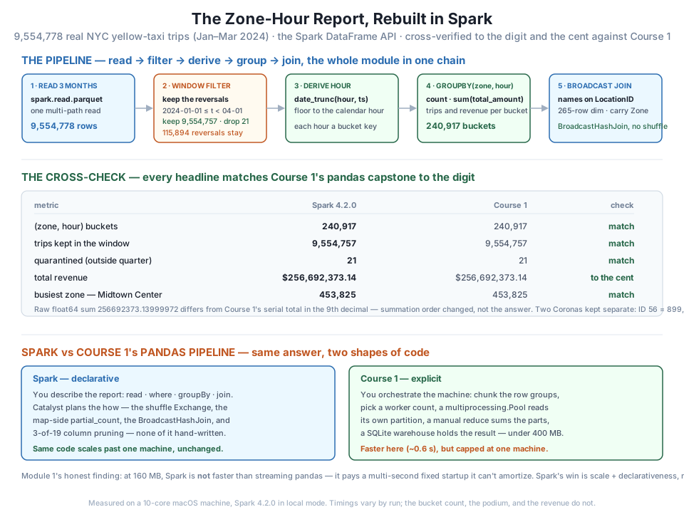
date_trunc the pickup hour → groupBy(PULocationID, pickup_hour).agg(count, sum) into 240,917 buckets → a BroadcastHashJoin that attaches names on LocationID with no extra shuffle. The cross-check (band two) holds to the digit against Course 1: 240,917 buckets, 9,554,757 trips, 21 quarantined, the podium led by Midtown Center at 453,825, the two Coronas distinct at 899 and 35 — and revenue to the cent, $256,692,373.14, even though the raw float64 sum (256692373.13999972) differs in the ninth decimal because the summation order changed, not the answer. Band three contrasts the declarative Spark job with Course 1's explicit pandas-plus-multiprocessing pipeline: same answer, and — per Module 1's honest finding — not faster at this 160 MB scale, but the one whose code scales past the machine.Two courses, two engines, one answer to the cent. It is worth setting the code side by side, because the shape of the two pipelines is the real lesson — not which is faster.
Course 1’s aggregator, at its core, told the machine how to do the work: read a specific row group, pull three columns into NumPy, filter on an explicit datetime comparison, group with pandas, and — the part that made it scale on one machine — hand each (path, row_group) to a multiprocessing worker that read its own partition and returned a tiny aggregate, which a manual reduce step then summed.
# gate: skip
# Course 1's shape (pandas + multiprocessing): YOU orchestrate the parallelism.
def aggregate_partition(task):
    path, rg = task
    tbl = pq.ParquetFile(path).read_row_group(rg, columns=KEEP)
    ts = tbl.column(0).to_numpy(zero_copy_only=False)         # datetime64[us]
    keep = (ts >= np.datetime64(WIN_LO)) & (ts < np.datetime64(WIN_HI))
    hour = ts[keep].astype("datetime64[h]").astype("int64")   # bucket key
    zone = tbl.column(1).to_numpy()[keep]
    amt  = tbl.column(2).to_numpy(zero_copy_only=False)[keep]
    return (pd.DataFrame({"zone": zone, "hour": hour, "amt": amt})
            .groupby(["zone", "hour"], sort=False)
            .agg(trips=("amt", "size"), revenue=("amt", "sum")).reset_index())

with mp.Pool(processes=6) as pool:            # you choose the workers
    parts = pool.map(aggregate_partition, tasks_for(FILES))
final = reduce_parts(parts)                   # you write the reduce
The Spark version, which you built in Steps 3–6, told the engine what the report is and let it decide how:
# gate: skip
# The Spark shape (DataFrame API): you describe the report; Catalyst plans the how.
in_window = trips.where((F.col("tpep_pickup_datetime") >= LO) &
                        (F.col("tpep_pickup_datetime") < HI))
report = (in_window
          .withColumn("pickup_hour", F.date_trunc("hour", "tpep_pickup_datetime"))
          .groupBy("PULocationID", "pickup_hour")
          .agg(F.count("*").alias("trips"), F.sum("total_amount").alias("revenue"))
          .join(broadcast(zones), F.col("PULocationID") == F.col("LocationID"), "left"))
Read the plan from Step 6 again with the two side by side, and the trade is concrete. The things Course 1 wrote by hand — split the files into partitions, pick a worker count, read each partition in its own process, reduce the partial aggregates, decide which table is small enough to broadcast — are all in Spark’s physical plan instead: the Exchange is the shuffle Spark chose for the group-by, the partial_count/partial_sum are the map-side pre-aggregation it inserted automatically, the BroadcastHashJoin is the small-table optimization it decided on from the 265-row size, and the ReadSchema of three columns out of nineteen is column pruning you never asked for. You described the report; Catalyst wrote the execution.
What each buys is a fair trade, not a verdict. Course 1’s pipeline is explicit and budget-controlled: you can see and cap every megabyte, which is exactly why it held under 400 MB while the naive load blew past a gigabyte — and on one machine, at this scale, it is faster. Module 1’s Lesson 4 measured this honestly and did not flinch: streaming pandas produced this very report in about 0.6 s warm, while Spark pays a multi-second fixed startup bill it cannot amortize on 160 MB of data. If the job is “aggregate one quarter and exit,” Spark is the slower tool, and pretending otherwise would waste everything Course 1 taught about measuring before believing.
Spark’s win is on a different axis. The declarative code is shorter, and it does not encode the machine: there is no worker count, no partition loop, no reduce, no memory budget — because the same groupBy and broadcast run unchanged on ten cores here or ten thousand across a cluster, against a quarter that fits in RAM or a decade that does not. Course 1’s pipeline is capped by the one machine it was hand-tuned for; the moment the data outgrows that machine, its explicit multiprocessing.Pool cannot follow, and the Spark job simply gets more executors. That is the whole reason this course exists after Course 1: not because Spark is faster on data that fits — it is not — but because the code you just wrote is the code that keeps working when the data stops fitting.
Same answer, different last bits — and why that’s the honest result
Spark summed the quarter’s revenue to 256692373.13999972; Module 1’s Spark job got 256692373.14026505; Course 1’s serial pandas total was a third value. All three round to $256,692,373.14. This is not a defect — it is float64 addition being non-associative, so the order of nine and a half million additions (which grouping and parallelism both change) moves the result by a fraction of a cent. The right response is the one this project practiced: sum in float64, round explicitly, and cross-check against an independent computation. When cents are contractually binding — invoicing, audited reconciliation — you sum in integer cents or decimal instead. For an analytics report checked against a known baseline, agreement after rounding by a comfortable margin is the standard, and getting it from an engine that added the numbers in a different order than pandas did is stronger evidence of correctness, not weaker.
Why the join added no shuffle
The plan in Step 6 has exactly one Exchange — the group-by’s shuffle — and none for the join. That is broadcast(zones) at work: because the dimension is 265 rows, Spark ships a copy to every executor and joins each aggregated row against the local copy, turning what would otherwise be a second full shuffle (a SortMergeJoin) into a BroadcastHashJoin. On this data the difference is small — the aggregated side is only 240,917 rows — but the habit matters: attaching a small dimension to a large fact table is the single most common join in analytics, and broadcasting the small side is how you keep it from dominating the job. Key it on the ID (LocationID), not the name, or the two Coronas fuse.
These extend the report. Keep the runnable blocks above intact — each exercise builds on the spark session and the pipeline functions.
Exercise 1 — Add the busiest single zone-hours. The report is a (zone, hour) table, so its most extreme rows are individual rush hours. Sort the named report by trips descending and print the top three (zone, hour) buckets with their trip counts and revenue. Course 1’s warehouse found the busiest single hours were around bar-close in the East Village and rush hour in Midtown — confirm your top row is a plausible surge and name the zone, the date, and the hour.
Hint
You already have named (buckets joined to names) — no re-aggregation needed, because the report is already at (zone, hour) grain. named.orderBy(F.desc(“trips”)).select(“Zone”, “pickup_hour”, “trips”, “revenue”).show(3, truncate=False). The pickup_hour column is a full timestamp truncated to the hour, so it names the exact hour directly — no decoding needed, unlike Course 1’s hours-since-epoch integer. Expect the top rows to be single hours with several hundred trips; a whole-day zone total is in the hundreds of thousands, so don’t confuse the two grains.
Exercise 2 — Prove the reversal policy changes the podium’s revenue, not its ranking. Rebuild the per-zone totals a second time from a frame that drops the negatives (where(total_amount >= 0)), and compare the top five’s revenue against the correct version. Confirm the ranking by trips is unchanged (dropping negatives removes no trips from the count in a way that reorders the top five) but the revenue is inflated, and report JFK’s revenue difference in dollars.
Hint
Trips are a count, so dropping the void half of a reversal pair changes a zone’s count only by the number of negative rows it holds — usually too few to reorder the top five — but it changes revenue by the full value of the uncancelled charges. Build both versions with the same groupBy and join, then subtract. This is the podium-level echo of Step 3’s $2,986,808.76 quarter-wide inflation: the error concentrates in the busy zones, and a reviewer eyeballing “the ranking looks right” would never catch it. Comparing revenue, format to two decimals first — raw float64 equality will fail on the last bits.
Exercise 3 — Turn off the broadcast and read the difference in the plan. Rebuild the join without broadcast() — a plain report.join(zones, ...) — and call .explain() on both. Compare the physical plans: identify the join operator each one chose and count the Exchange (shuffle) nodes in each. Explain in a sentence why, at 265 dimension rows, the broadcast is the right call, and note whether Spark’s Adaptive Query Execution might have broadcast the small side anyway.
Hint
Without the hint, Spark decides the join strategy from its size estimate: below spark.sql.autoBroadcastJoinThreshold (10 MB by default) it may broadcast on its own, so you might see a BroadcastHashJoin even without the explicit call — the 265-row CSV is far under the threshold. Force the contrast by reading the plan for what it commits to: the explicit broadcast() is a guarantee, not a suggestion, which matters when a dimension is near the threshold or when statistics are missing (as they are on these unsorted, stats-free Parquet files). Count the Exchange nodes: a shuffle join adds one on each side; the broadcast adds a BroadcastExchange on the small side only and leaves the big side where it is.
You rebuilt Course 1’s entire zone-hour report in idiomatic Spark and held it to an answer key. One multi-path read.parquet pulled all three months — 9,554,778 rows — into a single DataFrame. A window filter over kept 9,554,757 trips and quarantined exactly 21, while preserving all 115,894 in-window fare reversals — because dropping the negatives would have inflated revenue by $2,986,808.76, three million dollars of error the “clean the data” instinct invites. F.date_trunc("hour", ...) labelled each trip with its calendar hour, and groupBy(PULocationID, pickup_hour).agg(count, sum) produced exactly 240,917 buckets whose trips summed back to 9,554,757 and whose revenue rounded to $256,692,373.14 — from a raw float64 sum (256692373.13999972) whose last bits differ from both Course 1’s serial total and Module 1’s own Spark run, because the summation order changed, not the answer. A broadcast() join attached names from the 265-row dimension on LocationID with no extra shuffle (a BroadcastHashJoin in the plan), keeping the two Queens “Corona” zones distinct at 899 and 35 trips, and the busiest-zone podium matched to the digit — Midtown Center 453,825, then Upper East Side South, JFK (first by revenue at $33.1M), Upper East Side North, and Midtown East. All of it ships as cityflow_zone_hour_report.py: functions, a main(), a printed page with 9 of 9 live cross-checks, and spark.stop(), built in 8.9 s on a warm session. And the closing contrast made the point of the whole course concrete: the same answer as Course 1’s pandas-plus-multiprocessing pipeline, from code that describes the report instead of orchestrating the machine — not faster at 160 MB, but the version that scales past the one machine Course 1 was tuned for.
read → where(window) → withColumn(date_trunc hour) → groupBy(id, hour).agg(count, sum) → join(broadcast(dim)) is Lessons 1–4 assembled; each stage is a piece an earlier lesson left, and the value is in how they compose into one verified report.where keeps every in-window reversal; a total_amount >= 0 “cleanup” would delete the void halves and inflate revenue by $2,986,808.76, because reversals cancel inside SUM only when both halves survive.date_trunc("hour", ts) makes each calendar hour a distinct bucket (240,917 of them); hour(ts) would collapse the quarter into 24 buckets per zone and answer a different question.PULocationID keeps the two “Corona” zones separate (899 vs 35), and broadcast() attaches the 265-row dimension with a BroadcastHashJoin that adds no shuffle to the plan.This lesson is the module’s thesis proved on real data: fluency in the DataFrame API is the ability to write a correct report from scratch, on data that fights back, and know it is correct because a system you already trust says the same thing. CityFlow’s team could have rewritten this report in Spark and shipped it the moment it “looked right” — a familiar podium, revenue in the right hundreds of millions — and been silently wrong by three million dollars if a reviewer had waved through a where(total_amount >= 0), or wrong about two neighborhoods if the join had keyed on a name. The defense is the one this project practiced end to end: carry the old system’s verified numbers into the new one as executable checks at the finest grain you can afford, and treat a mismatch as a bug to investigate, never a rounding detail to paper over. That discipline is what makes the migration trustworthy — and the reason to make it at all is the honest trade the closing section drew: Spark is not faster than a hand-tuned pandas pipeline on data that fits one machine, but it is the only version of this report whose code does not have to be rewritten when the data no longer does.
That completes Module 3: DataFrames & Transformations — the DataFrame API as CityFlow’s daily tool. You built derived columns with lazy expressions, filtered and cleaned the taxi data’s real dirt without corrupting a total, joined the zone dimension with a broadcast that skips the shuffle, grouped and aggregated per zone and per hour, and here assembled all four into the report that pays off the module and Course 1 at once — cross-verified to the digit and to the cent.
But look again at the plan you read in Step 6, because it holds the next module’s whole subject. You wrote Python — groupBy, agg, broadcast — and Spark answered with a physical plan full of things you never typed: an Exchange, a partial_count, a BroadcastHashJoin, a three-column ReadSchema pruned from nineteen. Module 4 — Spark SQL & Execution Plans — turns that relationship around. You’ll express this exact report as a SQL query against a registered view and watch it compile to the same plan the DataFrame API produced, because both are front ends to Catalyst. Then you’ll read those plans deeply — the difference between the parsed, analyzed, optimized, and physical stages; what Exchange, AQEShuffleRead, and pushed filters actually cost; and how to spot the shuffle you didn’t need before it spots you. Once you can read the plan, you stop writing Spark by hope and start writing it by prediction — which is exactly what the last two modules have been building you toward.
Keep DATATWEETS free. Help fund practical data, AI, and engineering lessons for learners worldwide.
