Title here
Summary here
Module 4 left CityFlow’s team staring at the one thing Catalyst refused to optimize away: the Exchange under the zone-hour report, the shuffle that grouping by key genuinely requires. The question it handed forward was not “how do I delete this shuffle?” but “how big is it, and can I make it cheaper?” Every honest answer to that question runs through a single number that almost nobody looks at — the partition count — because a shuffle’s size, a stage’s parallelism, and a job’s scheduling overhead are all downstream of how many pieces the data is cut into. This module is where Spark tuning stops being about the query you wrote and starts being about the machine underneath it, and it begins here, with the piece.
This lesson proves four things on the real January yellow-taxi month, each measured rather than asserted. First, that a partition is the unit of parallelism — Spark schedules exactly one task per partition per stage, so the count is the ceiling on how many of your 10 cores can work at once. Second, that CityFlow’s month reads as exactly 10 partitions, and why — a split-sizing rule you can compute by hand and then confirm by moving the knob. Third, that the two tools for changing the count, repartition and coalesce, are not interchangeable: one is a full shuffle and one moves no data at all, a difference you can read straight off the physical plan. And fourth, that partition count has a Goldilocks curve — too few starves your cores, too many drowns the job in scheduling — with a sweet spot you can measure. Through all of it, one fact holds like a plumb line: the trip count stays 2,964,624 no matter how you slice the data.
By the end of this lesson, you will be able to:
df.rdd.getNumPartitions(), tying it back to the tasks from Module 2’s DAG lessonspark.sql.files.maxPartitionBytes, defaultParallelism, and the split-sizing formula — then confirm it by shrinking the caprepartition(n) (a full shuffle, even sizes, raises or lowers the count) and coalesce(n) (no shuffle, merges neighbours, only lowers it) and point at the Exchange vs Coalesce node that proves which ranrepartition(col) to hash-partition by a key and see every row for one zone land in a single partition, previewing the shuffle that groupBy and join will spend Lesson 2 onYou’ll need pyspark (JDK 17 or 21 — see the course setup) and the three taxi-quarter Parquet files. No new packages; getNumPartitions and .explain() are built into every DataFrame.
Before touching a knob, fix the idea. When Spark reads your data it splits it into partitions — contiguous chunks of rows — and a partition is the smallest thing Spark ever hands to a core. For each stage of a job, Spark launches one task per partition: a task is the work of running that stage’s operators over exactly one partition. That is the whole mechanism from Module 2’s job/stage/task lesson, stated as a rule you can now act on: partition count is the ceiling on parallelism. Ten partitions can keep ten cores busy; two partitions leave eight cores idle no matter how many you own; a thousand partitions on ten cores means each core works through a hundred tiny tasks in sequence, paying the fixed cost of launching each one.
So the first thing to know about any DataFrame is how many partitions it has. Start the standard session and open one month — CityFlow’s January — then ask:
# gate: skip
# CityFlow's verified quarter, fetched once from the public TLC source.
import urllib.request
for month in ("01", "02", "03"):
    urllib.request.urlretrieve(
        f"https://d37ci6vzurychx.cloudfront.net/trip-data/yellow_tripdata_2024-{month}.parquet",
        f"yellow_tripdata_2024-{month}.parquet",
    )
import warnings
warnings.filterwarnings("ignore")
from pyspark.sql import SparkSession
import pyspark.sql.functions as F
spark = (SparkSession.builder
.appName("cityflow")
.master("local[*]")
.config("spark.ui.showConsoleProgress", "false")
.getOrCreate())
spark.sparkContext.setLogLevel("ERROR")
jan = spark.read.parquet("yellow_tripdata_2024-01.parquet")
print("partitions :", jan.rdd.getNumPartitions())
print("rows :", f"{jan.count():,}")
print("defaultParallelism:", spark.sparkContext.defaultParallelism)partitions : 10
rows : 2,964,624
defaultParallelism: 10Three numbers worth holding onto. The month is 2,964,624 trips — Course 1’s verified January count, unchanged — split across 10 partitions, and this machine’s defaultParallelism is 10 because it has 10 cores available to local[*]. When CityFlow runs any stage over jan, Spark launches 10 tasks, one per partition, and all 10 cores run at once. That the partition count and the core count are both 10 is not a coincidence, and unpacking why is the next section.
Ten partitions for a 47.6 MB file surprises people twice. Why not 1 — the file easily fits under the 128 MB cap you may have heard governs partition size? And why exactly 10? Both answers fall out of the one formula Spark uses to size file splits. Two configs feed it:
print("maxPartitionBytes:", spark.conf.get("spark.sql.files.maxPartitionBytes"))
print("openCostInBytes  :", spark.conf.get("spark.sql.files.openCostInBytes"))
maxPartitionBytes: 134217728b
openCostInBytes : 4194304bspark.sql.files.maxPartitionBytes is 134217728 bytes — exactly 128 MiB — the cap on how big one split may be. openCostInBytes is 4 MiB, Spark’s estimate of the fixed cost of opening a file, which it also uses as a floor so it never makes absurdly tiny splits. The split size Spark actually picks is:
where bytesPerCore spreads the data evenly across your cores:
Put the January numbers in. The file is 47.6 MiB, so bytesPerCore is roughly . Then maxSplitBytes = min(128 MiB, max(4 MiB, 5.16 MiB)) = 5.16 MiB. Cut a 47.6 MiB file into 5.16 MiB splits and you get about 10 of them. The 128 MiB cap never entered into it — it sits ten times higher than the split we landed on. On a file this size, it is defaultParallelism that decides the count, precisely so every core gets a share; the cap only bites on files large enough that totalBytes / cores would exceed 128 MiB.
That is a claim you can test rather than trust. If the cap truly isn’t binding at 128 MiB, then shrinking it below bytesPerCore should suddenly make it bind and raise the partition count:
for cap in ["134217728b", "4m", "2m", "1m"]:
    spark.conf.set("spark.sql.files.maxPartitionBytes", cap)
    df = spark.read.parquet("yellow_tripdata_2024-01.parquet")
    print(f"maxPartitionBytes={cap:12s} -> partitions = {df.rdd.getNumPartitions()}")

spark.conf.set("spark.sql.files.maxPartitionBytes", "134217728b")  # restore the default
maxPartitionBytes=134217728b -> partitions = 10
maxPartitionBytes=4m -> partitions = 12
maxPartitionBytes=2m -> partitions = 24
maxPartitionBytes=1m -> partitions = 48Exactly the behaviour the formula predicts. At the 128 MiB default the cap is dead weight and the count stays 10. Drop it to 4 MiB — now below the 5.16 MiB bytesPerCore, so the cap wins the min — and 47.6 MiB / 4 MiB gives 12. Halve it again to 24, and again to 48: the count tracks fileBytes / cap as soon as the cap is what binds. You’ve just watched the two levers trade off — defaultParallelism sets the floor of parallelism, maxPartitionBytes caps the size of any one piece, and the smaller constraint wins. (The same rule is why the 3-file, 160 MB quarter also plans 10: more bytes, but divided by the same 10 cores.)
This is a read-time decision, not a property of the file
Nothing about the Parquet file “contains” 10 partitions — the count is computed when Spark plans the scan, from the file size, the two configs above, and the cores available to this session. Run the same read on an 8-core laptop and you’d get a different count. That is why partition tuning is a property of how you run, not what you stored, and why local[2] (Module 2) re-planned the same data to fewer partitions: fewer cores, larger bytesPerCore, fewer splits.
repartition vs coalesceTen is what the reader gave you; it is not what every downstream step wants. Spark offers two tools to change the partition count, and the difference between them is the single most important thing in this lesson because it is the difference between moving data and not. Watch what each does to the count first:
print("start          :", jan.rdd.getNumPartitions())
print("repartition(20):", jan.repartition(20).rdd.getNumPartitions())
print("repartition(4) :", jan.repartition(4).rdd.getNumPartitions())
print("coalesce(4)    :", jan.coalesce(4).rdd.getNumPartitions())
print("coalesce(20)   :", jan.coalesce(20).rdd.getNumPartitions())
start : 10
repartition(20): 20
repartition(4) : 4
coalesce(4) : 4
coalesce(20) : 10The last line is the tell. repartition(20) raised the count to 20; repartition(4) lowered it to 4; repartition goes either direction. coalesce(4) lowered it to 4 like repartition did — but coalesce(20) did nothing, leaving it at 10. coalesce can only lower the count; ask it to raise the count and it silently ignores you. That asymmetry is a direct consequence of how each one works, which the physical plan spells out. Here is repartition(4):
jan.repartition(4).explain()== Physical Plan ==
AdaptiveSparkPlan isFinalPlan=false
+- Exchange RoundRobinPartitioning(4), REPARTITION_BY_NUM, [plan_id=121]
+- FileScan parquet [VendorID#0,tpep_pickup_datetime#1,...,Airport_fee#18] Batched: true, ..., Location: InMemoryFileIndex(1 paths)[[...]], ReadSchema: struct<...>(The 19-column list and the Location path are shortened to [...]; nothing else is changed.) There it is, right above the scan: an Exchange — the same node you learned in Module 4 to read as a shuffle. repartition is a full shuffle: every row is sent through the network to a new partition, and RoundRobinPartitioning(4) means Spark deals rows out to the 4 targets round-robin, like dealing cards, so the results come out evenly sized. That even balance is what you pay the shuffle for. Now coalesce(4):
jan.coalesce(4).explain()== Physical Plan ==
Coalesce 4
+- *(1) ColumnarToRow
+- FileScan parquet [VendorID#0,tpep_pickup_datetime#1,...,Airport_fee#18] Batched: true, ..., Location: InMemoryFileIndex(1 paths)[[...]], ReadSchema: struct<...>No Exchange. Instead a plain Coalesce 4 node sits over the scan. coalesce moves no data across the network at all — it just tells some tasks to read several of the original partitions in sequence, stitching 10 partitions into 4 by grouping them. That is why it’s cheap, why it can only reduce (you cannot stitch 10 partitions into 20 without splitting, which needs a shuffle), and why the pieces can come out uneven — if you coalesce 10 into 4, some tasks inherit 3 original partitions and some 2. The whole trade in one line: repartition pays a shuffle to get even partitions and any count you want; coalesce skips the shuffle but can only merge, possibly unevenly.
The tidy rule — “use coalesce to reduce because it skips the shuffle” — is right often enough to be dangerous, because coalesce has a catch that the plan makes visible. Since coalesce inserts no shuffle boundary, its low partition count flows upstream into the work that feeds it. Coalesce a scan down to 1 partition and you haven’t just merged the output — you’ve told Spark to do the scan itself in a single task. Watch it on a filter that keeps only JFK Airport’s trips:
airport = jan.filter(F.col("PULocationID") == 132)          # JFK
print("JFK trips:", f"{airport.count():,}")

print("\n-- coalesce(1): the Coalesce swallows the scan --")
airport.coalesce(1).explain()
print("-- repartition(1): an Exchange keeps the scan parallel --")
airport.repartition(1).explain()
JFK trips: 145,240
-- coalesce(1): the Coalesce swallows the scan --
== Physical Plan ==
Coalesce 1
+- *(1) Filter (isnotnull(PULocationID#7) AND (PULocationID#7 = 132))
+- *(1) ColumnarToRow
+- FileScan parquet [...] PushedFilters: [IsNotNull(PULocationID), EqualTo(PULocationID,132)], ReadSchema: struct<...>
-- repartition(1): an Exchange keeps the scan parallel --
== Physical Plan ==
AdaptiveSparkPlan isFinalPlan=false
+- Exchange SinglePartition, REPARTITION_BY_NUM, [plan_id=133]
+- Filter (isnotnull(PULocationID#7) AND (PULocationID#7 = 132))
+- FileScan parquet [...] PushedFilters: [IsNotNull(PULocationID), EqualTo(PULocationID,132)], ReadSchema: struct<...>Look at where the Filter and FileScan sit. Under coalesce(1) they are inside the single coalesced partition — one task scans and filters all 47.6 MB serially. Under repartition(1) the Exchange SinglePartition is a boundary: the scan and filter run in the normal 10 parallel tasks below it, and only the small filtered result (145,240 rows) is funnelled into one partition above it. That structural difference is deterministic — it’s in the plan every time. Does it show up on the clock? Time both, taking the best of several runs:
import time
def best_count(df, label, reps=6):
    best = None
    for _ in range(reps):
        t = time.perf_counter(); df.count(); dt = time.perf_counter() - t
        best = dt if best is None else min(best, dt)
    print(f"{label:22s} {best:.3f}s")
    return best

jan.count()  # warm the OS file cache first
c = best_count(jan.filter(F.col("PULocationID") == 132).coalesce(1),    "coalesce(1)")
r = best_count(jan.filter(F.col("PULocationID") == 132).repartition(1), "repartition(1)")
print(f"coalesce/repartition = {c/r:.2f}x")
coalesce(1) 0.063s
repartition(1) 0.057s
coalesce/repartition = 1.11xHere the two are all but tied — coalesce(1) a hair slower, well inside run-to-run noise. And that is itself the lesson: on 47.6 MB served from the OS page cache, reading the file in one task versus ten barely registers, because the scan is nearly free either way. The serialization the plan reveals is real, but its cost scales with the work above the Coalesce — and on a page-cached toy file that work is tiny. Make the upstream expensive (a disk-bound read of many gigabytes, a heavy withColumn, a wide scan of hundreds of columns) and coalesce(1)’s “do it all in one task” becomes a genuine bottleneck while repartition(1) keeps the heavy part on all ten cores. So the honest rule is sharper than the slogan “coalesce is cheaper because it skips the shuffle”: coalesce is right when the work above it is already small — trimming the number of output files after an aggregation, where merging a handful of already-computed partitions costs nothing and a repartition would add a needless Exchange. When reducing partitions would strangle an expensive upstream stage down to one core, repartition earns its shuffle. Don’t time sub-second toy jobs to decide — read the plan: if a Coalesce sits on top of heavy work, be suspicious.
Everything so far has been about changing the count; this section is about choosing it. There is a real cost to too few partitions and a real cost to too many, and the only way to know the shape is to measure. We’ll run one fixed piece of work — the zone-hour aggregation, heavy enough that per-row CPU matters — across a spread of partition counts and time it. One discipline matters here: these are sub-second jobs on a page-cached file, so a single run is dominated by JVM jitter and garbage-collection pauses and can even come out backwards. Warm the generated code once, then take the best of several runs per count, which is the stable signal:
def agg_job(df):
    return (df.groupBy("PULocationID",
                       F.date_trunc("hour", "tpep_pickup_datetime").alias("h"))
              .agg(F.count("*").alias("trips"),
                   F.sum("total_amount").alias("rev"),
                   F.avg("trip_distance").alias("dist"))
              .count())

agg_job(jan)  # warm the generated code, throwaway

def sweep(df, label, reps=4):
    best, out = None, None
    for _ in range(reps):
        t = time.perf_counter(); out = agg_job(df); dt = time.perf_counter() - t
        best = dt if best is None else min(best, dt)
    print(f"{label:26s} nparts={df.rdd.getNumPartitions():5d}  buckets={out:6d}  {best:.3f}s")
    return best

b1    = sweep(jan.coalesce(1),          "coalesce(1)   too few")
b2    = sweep(jan.coalesce(2),          "coalesce(2)   too few")
b5    = sweep(jan.coalesce(5),          "coalesce(5)   near cores")
b10   = sweep(jan,                      "native(10)    sweet")
b1000 = sweep(jan.repartition(1000),    "repartition(1000) too many", reps=1)

print(f"\ncoalesce(1)   is {b1/b10:6.2f}x the sweet-spot time")
print(f"coalesce(2)   is {b2/b10:6.2f}x")
print(f"coalesce(5)   is {b5/b10:6.2f}x")
print(f"repart(1000)  is {b1000/b10:6.2f}x")
coalesce(1) too few nparts= 1 buckets= 77547 0.878s
coalesce(2) too few nparts= 2 buckets= 77547 0.635s
coalesce(5) near cores nparts= 5 buckets= 77547 0.328s
native(10) sweet nparts= 10 buckets= 77547 0.290s
repartition(1000) too many nparts= 1000 buckets= 77547 38.259s
coalesce(1) is 3.03x the sweet-spot time
coalesce(2) is 2.19x
coalesce(5) is 1.13x
repart(1000) is 132.06xThere is the curve, and it has exactly the shape the theory promises. Too few partitions starve cores: coalesce(1) ran about 3x slower and coalesce(2) about 2.2x slower, because one or two cores do all the aggregation while the other eight or nine sit idle — you own 10 cores and are using a fifth of them. The sweet spot is flat from 5 to 10 partitions, right around the core count: enough tasks to fill every core, few enough that scheduling is negligible (coalesce(5) is already within 13% of the best). And too many is catastrophic: repartition(1000) ran ~132x slower — not because the work grew (it’s the same 77,547 zone-hour buckets for the month either way) but because Spark had to shuffle the data into 1000 partitions and then schedule, launch, and tear down 1000 tiny tasks on 10 cores, a hundred sequential waves of pure overhead. The practical rule writes itself: partition count should be in the neighbourhood of your core count (a small multiple is fine), and the failure is far more painful on the high side than the low side. Absolute seconds vary run to run and machine to machine — the ratios and the shape are what transfer. And note the buckets never move: 77,547 for January in every row, the aggregation’s answer independent of how the input was split.
repartition(col): Partitioning by a KeyThere is a third form of repartition that this module’s next two lessons lean on, so meet it now. Pass a column instead of (or alongside) a number, and Spark doesn’t deal rows out round-robin — it hash-partitions by that key, sending every row with the same key value to the same partition. Do it on PULocationID and then look at where the rows landed, using spark_partition_id() to tag each row with its partition:
by_zone = jan.repartition(8, "PULocationID")

dist = (by_zone.withColumn("pid", F.spark_partition_id())
               .groupBy("pid")
               .agg(F.count("*").alias("rows"),
                    F.countDistinct("PULocationID").alias("zones"))
               .orderBy("pid"))
dist.show()

jfk_pids = (by_zone.withColumn("pid", F.spark_partition_id())
                   .filter(F.col("PULocationID") == 132)
                   .select("pid").distinct().collect())
print("JFK (132) lives in partition(s):", [r["pid"] for r in jfk_pids])
+---+------+-----+
|pid| rows|zones|
+---+------+-----+
| 0|479399| 28|
| 1|445765| 32|
| 2| 96742| 28|
| 3|359505| 44|
| 4|211262| 26|
| 5|574147| 40|
| 6|378257| 34|
| 7|419547| 28|
+---+------+-----+
JFK (132) lives in partition(s): [5]Two things to notice, both important for what’s coming. First, every JFK trip landed in exactly one partition (number 5) — that’s the defining property of hash-partitioning by a key: all rows sharing a key are colocated. That is precisely what a groupBy needs before it can total each zone, and what a join needs before it can match rows — which is why repartition(col) is a preview of the shuffle those operations perform for you automatically. Second, look at the rows column: the partitions are badly uneven, from 96,742 to 574,147. Hashing by a real-world key does not spread rows evenly, because keys don’t occur equally often — and that imbalance, when one key is enormous, is the skew that Lesson 4 is devoted to. Contrast this with a plain repartition(8), which deals round-robin and comes out dead even at 370,578 rows per partition. Partitioning by a column buys you colocation-by-key at the cost of even sizes; partitioning by a number buys you even sizes with no colocation.
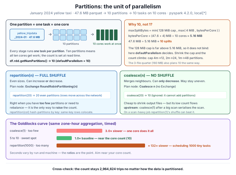
bytesPerCore (≈ 5.16 MiB) — not the 128 MiB cap — binds, so defaultParallelism = 10 decides. repartition(n) is a full shuffle (Exchange RoundRobinPartitioning, even, up or down); coalesce(n) is no shuffle (Coalesce, merge-only). The Goldilocks curve is real: coalesce(1) ran ≈ 3× slower, the sweet spot sits near 10, and repartition(1000) ran ≈ 132× slower. The count holds at 2,964,624.AQE reshapes shuffle partitions, but not these read partitions
Adaptive Query Execution (on by default in Spark 4) coalesces the post-shuffle partitions of a wide operation at runtime — that’s the 200-to-6 collapse you saw on the zone-hour report in Module 4. It does not touch the read partition count you get from a FileScan, nor override an explicit repartition/coalesce you asked for. This lesson’s counts — 10 from the read, 20 from repartition(20), 1000 from repartition(1000) — are all things you set directly; AQE’s job is the shuffle in the middle, which is Lesson 2’s subject.
One promise remains: that none of this reshaping changes the answer. Partitioning is purely about how the work is divided across cores, never what it computes. Hold the count against Course 1’s ground truth after slicing the data every way we’ve tried:
print("native   :", f"{jan.count():,}")
print("repart 20:", f"{jan.repartition(20).count():,}")
print("coalesce2:", f"{jan.coalesce(2).count():,}")
print("by zone  :", f"{jan.repartition(8, 'PULocationID').count():,}")

spark.stop()
print("session closed")
native : 2,964,624
repart 20: 2,964,624
coalesce2: 2,964,624
by zone : 2,964,624
session closedEvery partitioning gives 2,964,624 — Course 1’s verified January count, to the row. Partition count is a performance dial, not a correctness one: turn it for speed, and the result is exactly as safe as it was before you touched it.
Exercise 1 — Predict the count, then move the knob. Open the February month (yellow_tripdata_2024-02.parquet, 3,007,526 trips, about 49 MB on disk) and, before running anything, predict its partition count from the split-sizing rule. Then confirm with getNumPartitions(). Next, set spark.sql.files.maxPartitionBytes to "3m", re-read, and predict-then-check the new count. Finally reason out loud: on a machine with 4 cores instead of 10, would February’s default count go up or down, and why?
Hint
bytesPerCore = (fileBytes + 4 MiB) / defaultParallelism. For February that’s about MiB per split, and since that’s below the 128 MiB cap, expect 10 again — the count follows cores, not file size, until a file gets big. With the cap at "3m" the cap now binds (3 MiB is below 5.3 MiB), so predict roughly 49 MiB / 3 MiB ≈ 17. Fewer cores means a larger bytesPerCore (dividing by 4 instead of 10), so bigger splits and fewer partitions — the read follows the machine, exactly the point of the “read-time decision” callout.
Exercise 2 — Read the plan before you time it. Take jan.coalesce(3) and jan.repartition(3) and run .explain() on each. For each, write one sentence naming the top node (Coalesce vs Exchange RoundRobinPartitioning) and whether any data moves across the network. Then predict which will produce more evenly sized partitions, and verify with a spark_partition_id() row-count per partition like the one in the lesson. Did the coalesced version come out uneven? By how much?
Hint
repartition(3) shows an Exchange — a full shuffle, so its three partitions come out near-equal (about 988,000 rows each). coalesce(3) shows a Coalesce 3 and no Exchange — it stitches the original 10 read partitions into 3 groups without moving rows, so you’ll likely see something like 4+3+3 original partitions bundled together and correspondingly uneven row counts. The plan told you the shape before you measured it: no Exchange means no rebalancing, which means accept whatever unevenness the merge produces.
Exercise 3 — Find your machine’s sweet spot. Reproduce the Goldilocks sweep on the February month, but choose the partition counts to match your hardware: run the aggregation at 1, 2, at your core count, at twice your core count, and at 1000 partitions, timing each after a warm-up run. Plot or tabulate the times. Where is your flat sweet spot, and how many times slower is 1000 than the best count on your machine? Is the too-few penalty or the too-many penalty larger for you?
Hint
Warm the generated code once with a throwaway agg_job(feb) before timing, or your first measurement will absorb JIT cost and look artificially slow. Expect the flat region to sit around your core count and the 1000 case to be dramatically slower — on the lesson’s 10-core machine it was ~103x, dominated by scheduling a thousand tasks over ten cores. The exact ratios depend on your cores and disk, which is the whole point: the shape is universal, the numbers are yours. Report ratios, not raw seconds.
A partition is Spark’s unit of parallelism: the engine schedules exactly one task per partition per stage, so the partition count is the ceiling on how many cores can work at once. CityFlow’s January month reads as 10 partitions — and the split-sizing rule explains why: maxSplitBytes = min(maxPartitionBytes, max(openCostInBytes, bytesPerCore)), where bytesPerCore = (totalBytes + numFiles × openCostInBytes) / defaultParallelism. For a 47.6 MB file that’s about 5.16 MiB per split, so the file cuts into ~10 pieces; the 128 MiB maxPartitionBytes cap sits ten times higher and never binds, meaning defaultParallelism (10) sets the count — proven by shrinking the cap to 4m, 2m, 1m and watching the count climb to 12, 24, 48. Two tools reshape the count and the physical plan tells them apart: repartition(n) is a full shuffle (Exchange RoundRobinPartitioning, even sizes, raises or lowers the count) while coalesce(n) moves no data (a Coalesce node that merges neighbours, only lowers the count — coalesce(20) stayed 10). The convenient “coalesce is cheaper” rule has a trap the plan exposes: because coalesce adds no shuffle boundary, its low count flows upstream, so coalesce(1) runs the scan itself in one task while repartition(1)’s Exchange keeps the scan on all ten cores — a difference that was within timing noise on the page-cached 47.6 MB file (~1.1x) but grows with the size of the upstream work, which is why you read it in the plan rather than time it on toy data. Taking the best of several runs, the zone-hour aggregation across partition counts drew a real Goldilocks curve: coalesce(1) ran about 3x slower (starved cores), 5-10 partitions was the flat sweet spot near the core count, and repartition(1000) ran ~132x slower on shuffle-plus-scheduling overhead. Finally repartition(col) hash-partitions by key so every JFK trip landed in one partition (unevenly, from 96,742 to 574,147 rows) — a preview of the shuffle behind groupBy and join. Through all of it the count held at 2,964,624.
df.rdd.getNumPartitions(). Too few starves cores; too many buries the job in per-task scheduling.min(maxPartitionBytes, max(openCostInBytes, totalBytes/defaultParallelism)). On files small relative to 128 MiB × cores, defaultParallelism decides (the cap doesn’t bind), which is why 47.6 MB reads as 10 on a 10-core machine. It’s a read-time decision, not a property of the file.repartition(n) vs coalesce(n) — repartition is a full shuffle (Exchange), gives even partitions, and raises or lowers the count; coalesce is no shuffle (Coalesce), merges neighbours, can only lower the count, and may leave them uneven. Read the plan to know which ran.coalesce flows upstream — because it adds no shuffle boundary, a low coalesce count applies to the work feeding it, serializing an expensive scan onto few cores. repartition’s shuffle can be worth it when it keeps the upstream parallel; coalesce shines when the work above it is already small (trimming output files).coalesce(1) ran ~3x slower and repartition(1000) ran ~132x slower; the penalty is far worse on the high side. repartition(col) hash-partitions by key (colocation, but uneven), previewing the shuffle Lesson 2 dissects.Partition count is the number CityFlow’s engineers reach for first when a Spark job is slow, because it is upstream of almost everything else that costs time. A backfill crawling on one core is usually a coalesce that strangled the read; a job spending more time scheduling than computing is usually an over-eager repartition into thousands of tiny tasks; a shuffle that spills to disk is often a partition count mismatched to the cluster. Every one of those is now something you can see — read the count with getNumPartitions(), read the Exchange-or-Coalesce decision in the plan, and measure the curve rather than guess at it. And the discipline that makes it safe is the cross-check that closed the lesson: because partitioning changes only how work is divided and never what it computes, you can turn this dial as aggressively as the numbers justify and the answer stays 2,964,624 — correctness is free, only speed is on the table. That separation between what runs and how it runs on the machine is the whole premise of this module, and partitions are where it starts.
You’ve now met the shuffle three times without studying it head-on: as the Exchange that repartition inserts, as the boundary coalesce pointedly avoids, and as the key-based regrouping that repartition(col) performs to colocate every JFK trip in one partition. Lesson 2, Narrow vs Wide: the Shuffle, makes that regrouping the whole subject. You’ll draw the line between narrow transformations — map, filter, select, withColumn, where each output partition depends on exactly one input partition and no data moves — and wide ones — groupBy, join, distinct, orderBy, where rows must be regrouped across partitions and a shuffle is unavoidable. You’ll see what a shuffle physically is (partitioned files written to disk, moved across the network, read back), measure why it’s the single most expensive thing Spark does, and watch AQE coalesce those 200 configured shuffle partitions down to a handful — the runtime half of the partition story this lesson set up. Bring the plan-reading eye you sharpened here: every Exchange you learned to spot is a shuffle, and Lesson 2 is where you learn exactly what one costs.
Keep DATATWEETS free. Help fund practical data, AI, and engineering lessons for learners worldwide.
