Title here
Summary here
Module 4 left you with one operator you could not optimize away. You pruned columns, pushed filters, and folded constants until the zone-hour report’s plan was as lean as Catalyst could make it — and still, sitting in the middle of it, was a single Exchange. That Exchange is the shuffle, and Module 4’s last lesson named it as the one boundary the query needs by its very nature: to count trips per zone-hour, rows for the same bucket have to end up in the same place, and they start out scattered across ten partitions. Module 4 changed what runs. Module 5 is about how it runs on the machine underneath — and the shuffle is where that story begins, because it is, measurably, the most expensive thing Spark does.
This lesson gives you the vocabulary and the measurements to reason about it. Every transformation you write is either narrow — each output partition depends on exactly one input partition, so nothing moves — or wide — output partitions depend on many input partitions, so rows must be regrouped across the cluster, which is a shuffle. You will read that distinction straight off real plans (a narrow pipeline is one fused stage with no Exchange; a groupBy carries one), then take the shuffle apart at the mechanism level — write, transfer, read — and put a number on each part of it on CityFlow’s verified quarter. You’ll watch map-side pre-aggregation shrink 9,554,757 rows to 332,510 partial rows before any of them cross the wire, time a narrow pipeline against a wide one, and see adaptive query execution read the real post-shuffle size and coalesce the configured 200 partitions down to 6. The report will land, as always, on Course 1’s ground truth: 240,917 buckets, 9,554,757 trips, $256,692,373.14.
By the end of this lesson, you will be able to:
map, filter, select, withColumn) or wide (groupBy, join, distinct, orderBy, repartition) from the dependency between input and output partitionsExchange in a physical plan and name it as the shuffle, the stage boundary, and the query’s most expensive nodespark.sql.shuffle.partitions (default 200) and watch AQE override it downward from the real post-shuffle statisticsYou’ll need pyspark (JDK 17 or 21 — see the course setup) and the three taxi-quarter Parquet files. No new packages; every tool here is built into the DataFrame API and explain().
Start the standard session, stage the quarter, and hold the report window in a DataFrame we’ll reuse all lesson. Nothing here executes yet — these are transformations, building a plan:
import warnings; warnings.filterwarnings("ignore")
import time, statistics
from pyspark.sql import SparkSession, functions as F

spark = (SparkSession.builder
         .appName("cityflow")
         .master("local[*]")
         .config("spark.ui.showConsoleProgress", "false")
         .getOrCreate())
spark.sparkContext.setLogLevel("ERROR")

QUARTER = ["yellow_tripdata_2024-01.parquet",
           "yellow_tripdata_2024-02.parquet",
           "yellow_tripdata_2024-03.parquet"]
quarter = spark.read.parquet(*QUARTER)
windowed = quarter.filter(
    (F.col("tpep_pickup_datetime") >= "2024-01-01") &
    (F.col("tpep_pickup_datetime") < "2024-04-01"))

print("defaultParallelism           :", spark.sparkContext.defaultParallelism)
print("quarter partitions           :", quarter.rdd.getNumPartitions())
print("spark.sql.shuffle.partitions :", spark.conf.get("spark.sql.shuffle.partitions"))
defaultParallelism : 10
quarter partitions : 10
spark.sql.shuffle.partitions : 200Three facts to keep in front of us: this ten-core machine reads the quarter as 10 partitions, and spark.sql.shuffle.partitions — the configured task count for any stage downstream of a shuffle — is 200. Hold that 200; it is about to be both the number in the plan and the number the runtime refuses to obey.
Here is the whole distinction in one sentence. A narrow transformation is one where each output partition is built from exactly one input partition. A wide transformation is one where an output partition draws from many input partitions. That single dependency question — one parent or many — decides everything about cost, because “many parents” is only possible if rows physically move between partitions. Take a purely narrow pipeline — select off the windowed data — and read its plan:
narrow = windowed.select("PULocationID", "total_amount")
narrow.explain()
== Physical Plan ==
*(1) Project [PULocationID#7, total_amount#16]
+- *(1) Filter ((isnotnull(tpep_pickup_datetime#1) AND (tpep_pickup_datetime#1 >= 2024-01-01 00:00:00)) AND (tpep_pickup_datetime#1 < 2024-04-01 00:00:00))
+- *(1) ColumnarToRow
+- FileScan parquet [tpep_pickup_datetime#1,PULocationID#7,total_amount#16] Batched: true, PushedFilters: [IsNotNull(tpep_pickup_datetime), GreaterThanOrEqual(tpep_pickup_datetime,2024-01-01T00:00), Less..., ReadSchema: struct<tpep_pickup_datetime:timestamp_ntz,PULocationID:int,total_amount:double>(The FileScan line’s Location path and DataFilters are trimmed for width; nothing else changed.) Look at what is not there: no Exchange. FileScan, Filter, Project — scan, drop rows, drop columns — and every one of those reshapes a partition where it sits. The *(1) prefix on all three is Spark’s whole-stage code generation marker, and the fact that they share the number 1 is the plan telling you they fuse into one stage: Spark compiles filter-then-select into a single pass over each partition. Ten input partitions, ten output partitions, one-to-one, nothing crosses. This is the platonic narrow pipeline — it pipelines within a stage.
Now make one change that forces regrouping — group by zone and hour — and read the plan again:
report = (windowed
    .groupBy("PULocationID",
             F.date_trunc("hour", "tpep_pickup_datetime").alias("pickup_hour"))
    .agg(F.count("*").alias("trips"),
         F.sum("total_amount").alias("revenue")))
report.explain()
== Physical Plan ==
AdaptiveSparkPlan isFinalPlan=false
+- HashAggregate(keys=[PULocationID#7, _groupingexpression#44], functions=[count(1), sum(total_amount#16)])
+- Exchange hashpartitioning(PULocationID#7, _groupingexpression#44, 200), ENSURE_REQUIREMENTS, [plan_id=37]
+- HashAggregate(keys=[PULocationID#7, _groupingexpression#44], functions=[partial_count(1), partial_sum(total_amount#16)])
+- Project [PULocationID#7, total_amount#16, date_trunc(hour, cast(tpep_pickup_datetime#1 as timestamp), Some(Asia/Tehran)) AS _groupingexpression#44]
+- Filter ((isnotnull(tpep_pickup_datetime#1) AND (tpep_pickup_datetime#1 >= 2024-01-01 00:00:00)) AND (tpep_pickup_datetime#1 < 2024-04-01 00:00:00))
+- FileScan parquet [tpep_pickup_datetime#1,PULocationID#7,total_amount#16] ...(The FileScan line is path-shortened, as before.) There it is, dead center: Exchange hashpartitioning(PULocationID, _groupingexpression, 200). That Exchange is Spark’s plan-language for a shuffle, and it splits the plan in two. Everything below it — scan, filter, project, the first HashAggregate — is the map side, one stage. Everything above it — the final HashAggregate — is the reduce side, the next stage. groupBy is wide because to count all trips for zone 132, every zone-132 row (currently smeared across all ten partitions) has to arrive in one place first. join, distinct, orderBy, repartition are wide for the same reason and cut a stage the same way. This is exactly the tie-back to Module 2’s DAG lesson: every Exchange is a stage boundary, and counting the Exchanges in a plan is counting the shuffles.
Naming the shuffle is easy; the reason it dominates cost is worth understanding honestly, because you’ll spend the rest of this module minimizing it. A shuffle is a three-part physical operation, and it earns its expense in all three.
Shuffle write. Each map task finishes its slice of the scan and now holds rows it must hand off. It cannot just send them anywhere — every row has to reach the specific reduce partition responsible for its key. So the task computes, for each output row, hash(key) % numShufflePartitions, sorts its rows into that many buckets, and writes them to local files on disk — one region per target partition. Ten map tasks each writing 200 buckets’ worth of data means a lot of small, sorted, on-disk output. That write is real disk I/O, and it happens before a single row moves.
Network transfer. Now the data crosses the wire. On a real cluster the map tasks and reduce tasks live on different machines, so every reduce task must fetch its bucket from every map task — an all-to-all transfer, the map count times the reduce count in connections. This is the part that turns a shuffle from “some disk writes” into “the most expensive thing Spark does”: network bandwidth is the scarcest resource in a cluster, and a shuffle saturates it by design. (In local mode, “the network” is a loopback and the files are page-cached — which is exactly why our measurements below will be small and honest; the mechanism is what scales, not the seconds on one laptop.)
Shuffle read. Each reduce task pulls its assigned bucket from all the map outputs, merges them, and only now can it do its real work — the final aggregate, the join, the sort. It could not have started earlier: it needs every contributing row, and those rows were scattered until the transfer delivered them. That dependency — wait for all upstream partitions before producing any output — is the definition of a wide transformation, and it is why the shuffle is also a stage boundary: the reduce stage literally cannot begin until the map stage’s write has completed.
Write to disk, transfer across the network, read and merge — three times the data is touched, once on each side of a network hop. A narrow transformation touches each row once, in place. That is the entire cost difference, and everything in this module is a strategy to make the middle step move less.
Spark’s single most important defense against shuffle cost is already in the plan you read, and it has a name in the operators: partial_count(1) and partial_sum(total_amount), the map-side pre-aggregation. Look again at the two HashAggregate nodes in the wide plan — one below the Exchange, one above. The lower one runs on the map side, before the shuffle: each task builds a hash table keyed by (zone, hour) and accumulates a running count and sum per key it sees. A task that scanned a million rows but only saw a few thousand distinct zone-hours emits only a few thousand rows. The shuffle then moves those partials, not the raw rows, and the upper HashAggregate sums the partials into finished totals. You combine before you move.
Put a real number on how much that shrinks the shuffle. The rows crossing the Exchange are exactly the distinct (partition, zone, hour) combinations — one partial row per group per map task — so we can count them directly and hold them against the rows that entered:
n_in = windowed.count()

partials = (windowed
    .withColumn("part_id", F.spark_partition_id())
    .groupBy("part_id", "PULocationID",
             F.date_trunc("hour", "tpep_pickup_datetime").alias("bucket"))
    .count())
n_partials = partials.count()

print(f"rows entering the shuffle stage : {n_in:,}")
print(f"partial rows the shuffle writes : {n_partials:,}")
print(f"map-side pre-aggregation shrinks the shuffle {n_in / n_partials:.1f}x")
rows entering the shuffle stage : 9,554,757
partial rows the shuffle writes : 332,510
map-side pre-aggregation shrinks the shuffle 28.7x9,554,757 rows in, 332,510 rows across the wire — a 28.7x reduction, and every bit of it happened on the map side before the network was touched. Without pre-aggregation, all 9.5 million rows would have to be written, transferred, and read to be grouped on the other side; with it, the shuffle carries 3.5% of that. (The 332,510 partial rows are more than the 240,917 final buckets, because a bucket seen by three map tasks is written three times as three partials and only merged into one on the reduce side — the partials-to-buckets gap is the cost of ten tasks each summarizing independently.) This is why, back in Module 2, the shuffle write for a 9.5-million-row job was startlingly tiny: the job never moved 9.5 million rows. Hold this number when someone proposes a groupBy on a high-cardinality key — if every row is its own group, pre-aggregation buys nothing and the full dataset shuffles.
Now the cost that motivates the whole module: does a shuffle actually make the same work slower? Time a narrow-only pipeline (scan, filter, select, and a count whose final merge moves ten integers — one stage’s worth of real work) against the wide zone-hour groupBy (which cuts a genuine stage boundary and pays for the shuffle). Warm up first — a fresh session’s first job carries fixed startup cost we don’t want in the measurement — then take the median of several runs:
def bench(job, reps=5):
    job()  # warm up: pay one-time fixed costs before we start the clock
    times = []
    for _ in range(reps):
        t0 = time.perf_counter()
        job()
        times.append(time.perf_counter() - t0)
    return statistics.median(times), [round(t, 2) for t in times]

narrow_median, narrow_runs = bench(lambda: windowed.select("PULocationID", "total_amount").count())
wide_median, wide_runs = bench(lambda: report.count())

print(f"narrow one-stage pipeline : median {narrow_median:.2f}s   runs {narrow_runs}")
print(f"wide  one-shuffle pipeline: median {wide_median:.2f}s   runs {wide_runs}")
print(f"the shuffle adds roughly {wide_median / narrow_median:.1f}x")
narrow one-stage pipeline : median 0.24s runs [1.8, 0.24, 0.16, 0.23, 0.27]
wide one-shuffle pipeline: median 0.85s runs [1.37, 0.85, 0.75, 0.83, 0.98]
the shuffle adds roughly 3.6xThe wide pipeline costs about 3.6x the narrow one — a median 0.85s against 0.24s — reading the same rows off the same files. The only structural difference is the Exchange: the narrow job pipelines through one stage and returns; the wide job stops at the shuffle boundary, writes partials to disk, transfers them, reads them back, and finishes in a second stage. That whole write-transfer-read cycle is the extra 0.6 second.
Two honesties the numbers demand. First, look at the runs lists: the first timed run of each is an outlier (1.8s, 1.37s) even after a warm-up call — page caches, JIT compilation, and Spark’s own lazy initialization keep paying down for a job or two, which is exactly why we report the median, not the mean, and why seconds vary run to run and machine to machine. Second, and more important: this is a 160 MB job on one laptop where the shuffle files are page-cached and “the network” is a loopback. The ratio is the lesson, not the absolute seconds — a single-int-plus-double shuffle on this data is genuinely cheap. Move this to a real cluster with terabytes and a physical network between nodes, and that 3.6x becomes the difference between a query that finishes and one that doesn’t. The mechanism scales; the seconds on your laptop do not. That is the honest reason to spend a whole module learning to shrink shuffles you cannot remove.
One number in the wide plan was a lie waiting to be caught. The Exchange read hashpartitioning(..., 200) — the configured spark.sql.shuffle.partitions — which says the reduce side should run 200 tasks. Two hundred tasks to combine partials for 240,917 buckets that already fit in a few megabytes would be absurd: mostly-empty tasks, each with scheduling overhead, doing almost nothing. Spark 4 knows this, because adaptive query execution runs the map side first, measures the real size of the shuffle output, and re-sizes the reduce side from that measurement instead of the config’s guess. Force the report to execute and ask how many post-shuffle partitions it actually used:
print("post-shuffle partitions AQE chose:", report.rdd.getNumPartitions())
report.explain()
post-shuffle partitions AQE chose: 6
== Physical Plan ==
AdaptiveSparkPlan isFinalPlan=true
+- == Final Plan ==
ResultQueryStage 1
+- *(2) HashAggregate(keys=[PULocationID#7, _groupingexpression#44], functions=[count(1), sum(total_amount#16)])
+- AQEShuffleRead coalesced
+- ShuffleQueryStage 0
+- Exchange hashpartitioning(PULocationID#7, _groupingexpression#44, 200), ENSURE_REQUIREMENTS, [plan_id=1182]
+- *(1) HashAggregate(keys=[PULocationID#7, _groupingexpression#44], functions=[partial_count(1), partial_sum(total_amount#16)])
+- ... (map side, unchanged)
+- == Initial Plan ==
HashAggregate(keys=[PULocationID#7, _groupingexpression#44], functions=[count(1), sum(total_amount#16)])
+- Exchange hashpartitioning(PULocationID#7, _groupingexpression#44, 200), ENSURE_REQUIREMENTS, [plan_id=37]
+- ... (the draft you already read)(The map-side subtree and one FileScan path are trimmed; they are identical to the plan above.) The plan flipped isFinalPlan=false to true and split into == Final Plan == and == Initial Plan == — the draft it started with and the plan it actually ran. Sitting right above the Exchange is the new node: AQEShuffleRead coalesced, and it explains the printed count. The shuffle was written into 200 partitions, but AQE looked at the tiny real output and had each of just 6 reduce tasks read several of those 200 partitions’ worth of data, coalescing 200 down to 6. That is not a performance tweak you tuned; it is Spark 4’s default, and it is why the 200 in every hashpartitioning line of this course is a ceiling the runtime almost never hits.
To see that the 200 is genuinely the raw behavior AQE is overriding, switch adaptive execution off, rebuild the same report, and count again — then switch it straight back, because AQE-on is the real default:
spark.conf.set("spark.sql.adaptive.enabled", "false")
report_raw = (windowed
    .groupBy("PULocationID",
             F.date_trunc("hour", "tpep_pickup_datetime").alias("pickup_hour"))
    .agg(F.count("*").alias("trips"),
         F.sum("total_amount").alias("revenue")))
print("post-shuffle partitions with AQE off:", report_raw.rdd.getNumPartitions())
spark.conf.set("spark.sql.adaptive.enabled", "true")
post-shuffle partitions with AQE off: 200There is the config obeyed literally: 200 post-shuffle partitions, the number the Exchange printed all along, most of them nearly empty. spark.sql.shuffle.partitions is a single global knob applied to every shuffle in your application, and 200 is a historical default that fits neither a two-row group-by nor a two-billion-row one. AQE papers over that by right-sizing downward per shuffle from real statistics — but it can only coalesce, never split, and it can’t fix a value set absurdly low. Choosing that number deliberately, and knowing when AQE has your back and when it doesn’t, is Lesson 5’s tuning project; for now, the takeaway is that the shuffle’s width (200 or 6) is a thing you can see, and soon, set.
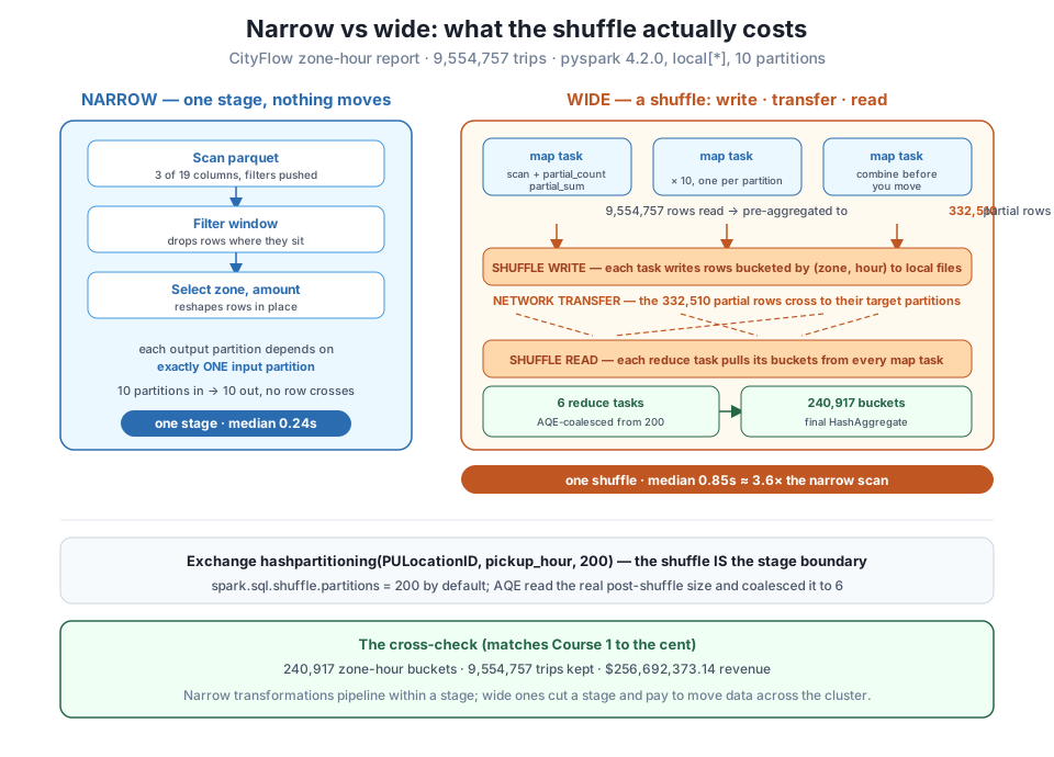
scan → filter → select fuse into one stage — each output partition depends on one input partition, nothing crosses, median 0.24s. Wide (right): the zone-hour groupBy is a shuffle — map tasks pre-aggregate 9,554,757 rows to 332,510 partials (28.7× smaller), write them bucketed by key, the partials transfer across the wire, and 6 reduce tasks (AQE-coalesced from spark.sql.shuffle.partitions = 200) read and combine them into 240,917 buckets, median 0.85s (≈ 3.6×). The report matches Course 1 to the cent: 9,554,757 trips, \$256,692,373.14.Confirm the shuffle computed the right answer, then close the session:
totals = report.agg(F.sum("trips").alias("t"), F.sum("revenue").alias("r")).first()
print(f"buckets : {report.count():,}")
print(f"trips   : {totals['t']:,}")
print(f"revenue : ${totals['r']:,.2f}")
spark.stop()
print("session closed")
buckets : 240,917
trips : 9,554,757
revenue : $256,692,373.14The shuffle moved 332,510 partial rows, coalesced to 6 reduce tasks, and produced Course 1’s verified report exactly — 240,917 buckets, 9,554,757 trips, $256,692,373.14. Same data, same answer, and now you can see and price the one operator that made it cost more than a scan.
Why the partials outnumber the buckets
The shuffle wrote 332,510 partial rows but the final report has 240,917 buckets — fewer, not more. There’s no contradiction: map-side pre-aggregation runs per task, so a zone-hour bucket that appears in three of the ten input partitions is summarized into three separate partial rows, one per task, and only merged into a single bucket on the reduce side after the shuffle delivers them together. The partials-to-buckets ratio (here about 1.38) measures how much each bucket was split across map tasks; a key that lived entirely in one partition would produce exactly one partial. It’s the price of letting ten tasks summarize independently before combining — and still a 28.7x win over shuffling the raw 9.5 million rows.
‘Pushed’ and ‘coalesced’ are runtime facts, not plan promises
The draft plan printed hashpartitioning(..., 200) and isFinalPlan=false; only after the query ran did the number become 6 and the flag become true. Get in the habit of reading a pre-run explain() as a forecast: it tells you the operators, where the shuffles are, and what the config requested — all decided at plan time and reliable. What it cannot tell you is what AQE will do with real statistics: how many partitions the shuffle coalesces to, or whether a join flips strategy. For that, run the query and re-read with isFinalPlan=true, or open the SQL tab of the Spark UI at localhost:4040, which draws the final plan after every action.
Exercise 1 — Classify, then confirm with the plan. For each of these five operations on windowed, write down first whether it is narrow or wide and how many Exchange nodes you expect, then run .explain() and check: (a) windowed.withColumn("tip_ratio", F.col("tip_amount") / F.col("total_amount")); (b) windowed.select("PULocationID").distinct(); (c) windowed.orderBy("total_amount"); (d) windowed.filter(F.col("total_amount") > 50); (e) windowed.repartition(8, "PULocationID"). Which ones carry an Exchange, and what partitioning does each Exchange use (hashpartitioning or rangepartitioning)?
Hint
Two are narrow — withColumn (a) and filter (d) reshape or thin rows in place, so their plans have no Exchange and everything shares one *(1) whole-stage tag. Three are wide: distinct (b) is secretly a groupBy on the selected column, so it carries a hashpartitioning Exchange; orderBy (c) has to range-slice the whole dataset, so its Exchange is rangepartitioning; and repartition(8, "PULocationID") (e) is a shuffle by definition — its entire job is moving rows — with a hashpartitioning(..., 8) Exchange where the 8 is the number you asked for, not the 200 default. Counting Exchanges is counting shuffles is counting stage boundaries.
Exercise 2 — Measure a shuffle you can’t pre-aggregate. The 28.7x win came from map-side pre-aggregation collapsing many rows per group. Build a groupBy where that barely helps — group by a near-unique key like F.col("tpep_pickup_datetime") (the raw microsecond timestamp) instead of the truncated hour — and count the partial rows the same way the lesson did (spark_partition_id(), group by (part_id, key), count the result), against the 9,554,757 input rows. What reduction do you get now, and why is it so much smaller than 28.7x? What does that tell you about which groupBy keys make a shuffle expensive?
Hint
Truncating to the hour created 240,917 groups from 9.5 million rows — heavy pre-aggregation, so each task emitted far fewer rows than it read. The raw timestamp has close to one distinct value per row, so each group is essentially a single row, each map task emits almost as many partial rows as it read, and the reduction collapses toward 1x — the shuffle carries nearly the full dataset. The rule to take away: pre-aggregation’s payoff scales with how many rows share a key, so a groupBy on a high-cardinality key (a timestamp, an id, a lat/long) shuffles roughly everything, while a groupBy on a low-cardinality key (a zone, a day, a category) shuffles a summary. Same operator, wildly different bill.
Exercise 3 — Watch AQE lose its grip. Rebuild the zone-hour report and, before running it, set spark.conf.set("spark.sql.shuffle.partitions", "4"). Force execution and print report.rdd.getNumPartitions(). Did you get 4, or did AQE still coalesce below it? Now set it to "500" and repeat. Compare both against the lesson’s default-200-coalesced-to-6 result, and decide: which knob is doing the work here, the config or AQE — and when would the config matter more than it does on this 160 MB job?
Hint
Setting the config to 4 makes the Exchange write only 4 partitions; AQE can coalesce (merge partitions downward) but never split, so it has nothing to shrink and you’ll likely see close to 4 — you undercut it. Setting it to 500 makes the Exchange write 500, and AQE coalesces that right back down toward the same handful it always wanted, so the post-shuffle count barely moves from the 6 you saw at 200. That’s the lesson: on this small job AQE dominates and the config is nearly irrelevant as long as it’s high enough to coalesce from. The config starts mattering when data is large enough that even the coalesced partitions are big — or when you set it too low and cap parallelism below what the data needs. Lesson 5 tunes exactly this trade-off; here you’re just proving AQE only ever shrinks.
Every transformation is narrow or wide, and the distinction is one question: does each output partition depend on one input partition or many? Narrow transformations (filter, select, withColumn) reshape rows in place, fuse into a single whole-stage-codegen stage, and move nothing — the narrow pipeline’s plan had no Exchange and one shared *(1) tag. Wide transformations (groupBy, join, distinct, orderBy, repartition) must regroup rows across the cluster, which is a shuffle — the zone-hour groupBy carried one Exchange hashpartitioning(..., 200), the shuffle and the stage boundary in a single node. A shuffle is expensive because it is three physical operations: map tasks write rows bucketed by key to local disk, the data transfers across the network in an all-to-all fetch, and reduce tasks read and merge their partition from every map task — three touches of the data around a network hop, versus a narrow transformation’s one touch in place. We measured all of it on CityFlow’s verified quarter: map-side partial_count/partial_sum pre-aggregation shrank the 9,554,757 windowed rows to 332,510 partial rows crossing the Exchange (28.7x, and more partials than the 240,917 final buckets because each task summarizes independently before the merge); a narrow filter-select-count ran a median 0.24s against the wide groupBy’s 0.85s (about 3.6x, honestly small on one page-cached 160 MB machine — the ratio and the mechanism scale, the seconds don’t); and adaptive query execution read the real post-shuffle size and coalesced the configured 200 partitions down to 6, showing its true colors as 200 only when we switched AQE off. The report cross-checked to Course 1 exactly: 240,917 buckets, 9,554,757 trips, $256,692,373.14.
filter, select, withColumn, map); no data moves, and chains of them fuse into a single stage that pipelines through each partition once. The cheap kind.groupBy, join, distinct, orderBy, repartition), so rows must be regrouped across the cluster. Every wide transformation forces a shuffle and cuts a stage. The expensive kind.Exchange = stage boundary — one node, three names. Physically it is shuffle write (map tasks bucket rows by key onto local disk), network transfer (all-to-all fetch), and shuffle read (reduce tasks merge their partition from every map task). It is the most expensive thing Spark does because it touches the data three times around a network hop.partial_count/partial_sum HashAggregate below the Exchange combines rows per key within each task before the shuffle, so only summaries cross the wire (9,554,757 → 332,510 here, 28.7x). Its payoff scales with rows-per-key: huge for low-cardinality keys, near-zero for near-unique ones.spark.sql.shuffle.partitions and AQE coalescing — the config sets the reduce-side task count for every shuffle (default 200); adaptive query execution overrides it downward per shuffle from real post-shuffle statistics (200 → 6 here), shown by AQEShuffleRead coalesced and isFinalPlan=true. AQE can only shrink, never split.CityFlow’s engineers don’t optimize pipelines by staring at wall-clock time — they find the shuffles and ask what crosses them. “This backfill groups by trip_id” is a red flag the moment you can read it, because a high-cardinality key defeats pre-aggregation and shuffles the entire fact table; “this groups by zone and day” is fine, because a few hundred keys means the shuffle carries a summary. That judgment is nothing more than the narrow/wide classification plus the pre-aggregation rule you drilled here, and it’s the difference between a query that scales to a cluster and one that quietly moves terabytes it didn’t need to. The measurements matter just as much as the vocabulary: on one 160 MB laptop a shuffle costs a fraction of a second and it’s tempting to dismiss it — but the 3.6x ratio, the write-transfer-read mechanism, and the 28.7x pre-aggregation win are all structural, and they’re exactly what turns into hours saved (or wasted) when the same code runs on real volumes. And reading spark.sql.shuffle.partitions against what AQE actually did keeps you honest about who controls parallelism: the config requests, the runtime decides, and knowing which knob is load-bearing at which scale is the whole content of this module’s tuning project.
This lesson priced the shuffle — the cost of moving data once. Lesson 3, Caching & Persistence, prices something subtler: the cost of computing the same data twice. Every DataFrame you’ve built is a lazy recipe, recomputed from source each time an action touches it — which means a windowed frame used by three separate reports scans and filters the quarter three times, paying the whole pipeline over on each. You met that twice-run trap back in Module 2; now you’ll fix it. You’ll cache() a reused DataFrame and measure the win when an iterative or multi-action workload stops recomputing, watch InMemoryTableScan appear in the plan where the recompute used to be, and — because this course tells the truth — you’ll also measure the case where caching hurts: a single-action job where the cache never pays for itself, or a frame too big to fit in memory, where Spark spills to disk and you’d have been faster without it. The question shifts from “how expensive is moving data?” to “when is it worth spending memory to avoid recomputing it?” Bring today’s instinct for measuring before believing — caching is a bet, and Lesson 3 teaches you to size the odds.
Keep DATATWEETS free. Help fund practical data, AI, and engineering lessons for learners worldwide.
