Title here
Summary here
Lesson 1 taught you that a partition is the unit of parallelism — one task per partition, ten tasks across CityFlow’s ten cores. Lesson 2 showed the shuffle that a groupBy forces, and Lesson 3 taught you when caching that shuffled input pays. Every one of those lessons quietly assumed something that is almost never true of real data: that the partitions are the same size. They are not. New York’s taxi trips do not spread themselves evenly across zones — a handful of airports and Midtown blocks generate a huge share of every pickup, and when Spark hash-partitions by pickup zone, those hot zones pile into a few partitions while most stay nearly empty. This lesson is about what happens next.
Here is the mechanism in one sentence, and it is the most important sentence in the module: a stage is only as fast as its slowest task. Spark runs one task per partition and the stage does not finish until the last task does, so if one partition holds thirteen times the rows of another, one task runs long while nine cores finish early and sit idle. That is a straggler, and it is the distributed-systems version of the plateau you measured in Course 1 — Amdahl’s law, where one un-parallelized fraction caps the speedup no matter how many cores you add. There the serial fraction was code that had to run on one thread; here it is data that has to run on one task. This lesson makes that skew visible on the real quarter, diagnoses it with a tool you already have, and works through the honest set of fixes — including the times a fix costs more than the problem.
By the end of this lesson, you will be able to:
F.spark_partition_id() — count rows per partition after a hash repartition and read the imbalance in actual numbersgroupBy)F.rand() to spread its rows across sub-partitions, run a two-stage aggregate, and verify the answer is unchangedYou’ll need pyspark and the three taxi-quarter Parquet files. No new packages — F.spark_partition_id, F.rand, and the built-in aggregates are all we use.
Before we can watch skew hurt, we have to establish that CityFlow’s data actually has a hot key — not as folklore, but as counts. Load the quarter, keep the report window, and hold onto just the two columns skew depends on: the shuffle key (PULocationID) and a value to aggregate (total_amount). We cache() this projection because every section below reuses it, exactly the reuse-pays situation Lesson 3 argued for.
import warnings
warnings.filterwarnings("ignore")
from pyspark.sql import SparkSession, functions as F

spark = (SparkSession.builder
         .appName("cityflow")
         .master("local[*]")
         .config("spark.ui.showConsoleProgress", "false")
         .getOrCreate())
spark.sparkContext.setLogLevel("ERROR")

FILES = ["yellow_tripdata_2024-01.parquet",
         "yellow_tripdata_2024-02.parquet",
         "yellow_tripdata_2024-03.parquet"]

trips = (spark.read.parquet(*FILES)
         .where((F.col("tpep_pickup_datetime") >= "2024-01-01") &
                (F.col("tpep_pickup_datetime") < "2024-04-01"))
         .select("PULocationID", "total_amount")
         .cache())

print("cores (defaultParallelism):", spark.sparkContext.defaultParallelism)
print("trips in the report window:", trips.count())
cores (defaultParallelism): 10
trips in the report window: 9554757Ten cores, and the module’s canonical 9,554,757 trips — the same count every lesson lands on. Now count trips per pickup zone and join the zone names so the hot key isn’t just a number:
zones = spark.read.csv("taxi_zone_lookup.csv", header=True, inferSchema=True)
per_zone = trips.groupBy("PULocationID").count()
labelled = (per_zone.join(zones, per_zone.PULocationID == zones.LocationID, "left")
                    .select("PULocationID", "Zone", "count"))

print("busiest pickup zones:")
labelled.orderBy(F.desc("count")).show(6, truncate=False)
print("quietest pickup zones:")
labelled.orderBy("count").show(6, truncate=False)
print("distinct pickup zones in the quarter:", per_zone.count())
busiest pickup zones:
+------------+-------------------------+------+
|PULocationID|Zone |count |
+------------+-------------------------+------+
|161 |Midtown Center |453825|
|237 |Upper East Side South |439138|
|132 |JFK Airport |429745|
|236 |Upper East Side North |416508|
|162 |Midtown East |336460|
|230 |Times Sq/Theatre District|331570|
+------------+-------------------------+------+
only showing top 6 rows
quietest pickup zones:
+------------+---------------------------------------------+-----+
|PULocationID|Zone |count|
+------------+---------------------------------------------+-----+
|105 |Governor's Island/Ellis Island/Liberty Island|1 |
|5 |Arden Heights |1 |
|204 |Rossville/Woodrow |1 |
|99 |Freshkills Park |2 |
|109 |Great Kills |2 |
|84 |Eltingville/Annadale/Prince's Bay |3 |
+------------+---------------------------------------------+-----+
only showing top 6 rows
distinct pickup zones in the quarter: 262There is the skew, in raw counts. Midtown Center at 453,825 trips and JFK Airport at 429,745 sit at the top — matching Course 1’s leaderboard to the trip — while Governor’s Island logged exactly one pickup all quarter. That is a range of nearly half a million to one across 262 zones. The distribution is not a gentle slope; it is a cliff. And critically, this is the shuffle key for the zone-hour report — the column Spark uses to decide which partition each row goes to. A key this lopsided is a straggler waiting to happen, because of one fact about hash partitioning we’re about to make painfully concrete: every row with the same key goes to the same partition. JFK’s 429,745 rows cannot be split across cores by a plain hash — they are one indivisible lump.
To see the imbalance as Spark’s scheduler sees it, force the exact partitioning a groupBy would use and then ask each partition how many rows it holds. df.repartition(10, F.col("PULocationID")) hash-partitions the trips by zone into ten partitions — one per core — and F.spark_partition_id() stamps each row with the partition it landed in. Group by that id and you have the per-task workload, measured:
by_key = (trips.repartition(10, F.col("PULocationID"))
               .withColumn("pid", F.spark_partition_id()))
sizes = by_key.groupBy("pid").count().orderBy(F.desc("count"))
sizes.show(10, truncate=False)
(sizes.agg(F.max("count").alias("max_rows"),
           F.min("count").alias("min_rows"),
           F.round(F.avg("count")).alias("avg_rows"),
           F.round(F.stddev("count")).alias("std_rows"),
           F.round(F.max("count") / F.min("count"), 1).alias("max_over_min"))
      .show())
+---+-------+
|pid|count |
+---+-------+
|3 |2278324|
|8 |1404036|
|4 |1095819|
|1 |1086779|
|7 |996312 |
|9 |758082 |
|5 |636269 |
|6 |570697 |
|0 |557798 |
|2 |170641 |
+---+-------+
+--------+--------+--------+--------+------------+
|max_rows|min_rows|avg_rows|std_rows|max_over_min|
+--------+--------+--------+--------+------------+
| 2278324| 170641|955476.0|582405.0| 13.4|
+--------+--------+--------+--------+------------+Read the top and bottom rows together, because that gap is the whole lesson. Partition 3 holds 2,278,324 rows; partition 2 holds 170,641 — a 13.4x spread around an average of 955,476, with a standard deviation (582,405) more than half the mean. When this stage runs, ten tasks launch at once. Nine of them chew through their share and finish; the task on partition 3 is still going, with more than double the average workload, and the stage cannot report done until it finishes. During that tail, most of your ten cores are idle. If you opened the Spark UI at http://localhost:4040 while this ran, the stage’s task table would show it directly: one task with far more input size and duration than the other nine, a long bar stretching past a cluster of short ones. That single long bar is the straggler, and it is why “we have ten cores” did not translate into “ten times faster.”
This is Amdahl’s plateau wearing new clothes. In Course 1’s parallelism lesson, the speedup ceiling came from a serial fraction — work that could not be split across workers. Here the “serial fraction” is partition 3: 2.28 million rows that must be processed by one task because they share hash buckets, no matter how many cores wait. Adding cores does not help; an eleventh core would sit idle too. The bottleneck is not the number of workers, it is the shape of the data.
It would be easy to assume partition 3 is just Midtown Center’s 453,825 rows. It is far more than that — 2.28 million — so something is stacking. Ask which zones actually landed on the biggest partition:
biggest_pid = sizes.first()["pid"]
print("biggest partition is pid", biggest_pid)
(by_key.where(F.col("pid") == biggest_pid)
       .groupBy("PULocationID").count()
       .join(zones, by_key.PULocationID == zones.LocationID, "left")
       .select("PULocationID", "Zone", "count")
       .orderBy(F.desc("count")).show(6, truncate=False))
biggest partition is pid 3
+------------+-------------------------+------+
|PULocationID|Zone |count |
+------------+-------------------------+------+
|237 |Upper East Side South |439138|
|236 |Upper East Side North |416508|
|138 |LaGuardia Airport |284359|
|141 |Lenox Hill West |229080|
|164 |Midtown South |215859|
|246 |West Chelsea/Hudson Yards|162058|
+------------+-------------------------+------+This is hash collision compounding skew. Partition 3 didn’t get one hot zone — it got both Upper East Side zones (439,138 and 416,508) plus LaGuardia (284,359) plus three more busy zones, because hash(PULocationID) % 10 happened to route all of them to bucket 3. Skew is bad enough when one hot key dominates a partition; it gets worse when the hash piles several hot keys together. Fewer partitions make this more likely (only ten buckets to spread 262 zones across), and no amount of “just pick a good number” fixes it reliably, because you cannot control which keys collide.
Does using more partitions help? Partly — but it trades one problem for another. Repartition by the same key into 200 (Spark’s default shuffle.partitions) and check the extremes:
wide = (trips.repartition(200, F.col("PULocationID"))
             .withColumn("pid", F.spark_partition_id())
             .groupBy("pid").count())
(wide.agg(F.max("count").alias("fattest"),
          F.min("count").alias("thinnest"),
          F.count("*").alias("non_empty"),
          F.lit(200).alias("configured"))
     .show())
+-------+--------+---------+----------+
|fattest|thinnest|non_empty|configured|
+-------+--------+---------+----------+
| 579093| 1| 145| 200|
+-------+--------+---------+----------+More partitions shrank the fattest one from 2.28 million to 579,093 — real relief, because fewer zones collide when there are 200 buckets. But look at the other two columns: only 145 of the 200 partitions hold any rows at all, and the thinnest holds a single row. So 55 tasks do nothing but pay their scheduling cost, and the fattest is still 579,093 rows — because a single hot key is indivisible, and even alone in its partition it outweighs the small ones by five orders of magnitude. More partitions is a real but blunt lever: it dilutes collisions, it cannot split a hot key.
Spark 4 ships Adaptive Query Execution on by default, and part of AQE is specifically a skew handler. Check what it’s configured to do:
for k in ("spark.sql.adaptive.enabled",
          "spark.sql.adaptive.skewJoin.enabled",
          "spark.sql.adaptive.skewJoin.skewedPartitionFactor",
          "spark.sql.adaptive.skewJoin.skewedPartitionThresholdInBytes"):
    print(f"{k} = {spark.conf.get(k)}")
spark.sql.adaptive.enabled = true
spark.sql.adaptive.skewJoin.enabled = true
spark.sql.adaptive.skewJoin.skewedPartitionFactor = 5.0
spark.sql.adaptive.skewJoin.skewedPartitionThresholdInBytes = 268435456bRead the setting name carefully: it is adaptive.**skewJoin**.enabled. At runtime, when a join produces shuffle partitions and one is both larger than skewedPartitionFactor (5.0) times the median and bigger than skewedPartitionThresholdInBytes (268,435,456 bytes — 256 MB), AQE splits that skewed partition into smaller pieces and replicates the matching rows from the other side, so several tasks share the hot partition’s work instead of one. For a skewed join, this is close to free: you get straggler relief with no code change, which is a genuinely big deal and one of the best reasons to keep AQE on.
But it is a join handler. A plain groupBy aggregation — CityFlow’s zone-hour report — is not covered by skewJoin, and even if it were, our fattest partition is 579,093 rows of two skinny int/double columns, nowhere near the 256 MB byte threshold. So AQE will happily coalesce our post-shuffle partitions (the 200-to-6 behavior from Lesson 2) without ever treating our skew as skew. The honest takeaway: AQE dissolves skew for the case it targets — large skewed joins — and leaves aggregation skew for you. Know which case you’re in before you reach for a manual fix.
If the problem is that all of a hot key’s rows share one bucket, the fix is to stop them sharing one bucket. Salting adds a small random integer — the salt — to the key, so a single zone becomes several sub-keys (JFK-0, JFK-1, …, JFK-7) that hash to different partitions. You aggregate on the salted key first (spreading the hot key’s work across tasks), then strip the salt and combine the partial results. The value column is untouched; only the grouping changes.
Build the salt with F.rand() — a built-in, no UDF — scaled to eight buckets, and check the balance the salted key produces when we repartition on it:
SALTS = 8
salted = trips.withColumn("salt", (F.rand(seed=7) * SALTS).cast("int"))
by_salted_key = (salted.repartition(10, F.col("PULocationID"), F.col("salt"))
                       .withColumn("pid", F.spark_partition_id()))
salted_sizes = by_salted_key.groupBy("pid").count().orderBy(F.desc("count"))
salted_sizes.show(10, truncate=False)
(salted_sizes.agg(F.max("count").alias("max_rows"),
                  F.min("count").alias("min_rows"),
                  F.round(F.stddev("count")).alias("std_rows"),
                  F.round(F.max("count") / F.min("count"), 1).alias("max_over_min"))
             .show())
+---+-------+
|pid|count |
+---+-------+
|1 |1144845|
|5 |1102580|
|6 |1063799|
|0 |1057413|
|8 |1004410|
|2 |921682 |
|9 |883685 |
|7 |852713 |
|3 |785004 |
|4 |738626 |
+---+-------+
+--------+--------+--------+------------+
|max_rows|min_rows|std_rows|max_over_min|
+--------+--------+--------+------------+
| 1144845| 738626|139428.0| 1.5|
+--------+--------+--------+------------+The imbalance collapses. Partitioning on (PULocationID, salt) instead of PULocationID alone drops the fattest partition from 2,278,324 to 1,144,845, tightens the standard deviation from 582,405 to 139,428 — a 4.2x tighter spread — and cuts the max-over-min ratio from 13.4x to 1.5x. Ten tasks now do roughly equal work; there is no straggler holding the stage open. The hot key is no longer indivisible, because we made eight of it.
But balance is worthless if it corrupts the answer. The salt was a means, not the result — so aggregate in two stages and strip it back off. Stage one counts by (zone, salt); stage two sums those partials by zone. The salt must vanish from the final numbers:
partial = salted.groupBy("PULocationID", "salt").count()
recombined = partial.groupBy("PULocationID").agg(F.sum("count").alias("trips"))
print("salted two-stage counts for the hot zones (must match the podium):")
recombined.where(F.col("PULocationID").isin(132, 161)).orderBy("PULocationID").show()
print("JFK's 429,745 trips, spread across 8 salt buckets:")
salted.where(F.col("PULocationID") == 132).groupBy("salt").count().orderBy("salt").show()
salted two-stage counts for the hot zones (must match the podium):
+------------+------+
|PULocationID| trips|
+------------+------+
| 132|429745|
| 161|453825|
+------------+------+
JFK's 429,745 trips, spread across 8 salt buckets:
+----+-----+
|salt|count|
+----+-----+
| 0|53955|
| 1|54064|
| 2|53705|
| 3|53597|
| 4|53913|
| 5|53721|
| 6|53160|
| 7|53630|
+----+-----+Exactly right. JFK comes back as 429,745 and Midtown Center as 453,825 — the podium numbers, to the trip — because summing the salted partials is arithmetically identical to counting the whole. And the second table shows why it balanced: JFK’s 429,745 trips split into eight buckets of roughly 53,700 each, so instead of one task carrying all of JFK, eight tasks carry a slice. That is the entire trick — spread on the way in, recombine on the way out, answer unchanged.
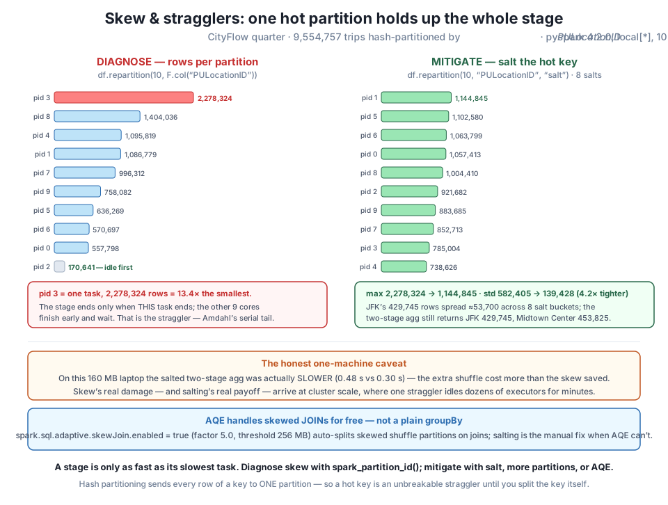
PULocationID into 10 partitions puts 2,278,324 rows on partition 3 and 170,641 on partition 2 — a 13.4× straggler (std 582,405) that holds the stage open while other cores idle. Right — salt: repartitioning on (PULocationID, salt) across 8 buckets drops the max to 1,144,845 and the spread to 1.5× (std 139,428, 4.2× tighter), spreading JFK’s 429,745 trips ≈53,700 per bucket — and the two-stage aggregate still returns JFK 429,745, Midtown Center 453,825. Honest coda: on this 160 MB machine the salted job ran slower (0.48 s vs 0.30 s); the payoff is at cluster scale. AQE’s skewJoin fixes skewed joins for free, never a plain groupBy.Salting is a targeted tool, not a default
Salt the key that is actually skewed, and only when skew is actually hurting — not every groupBy. The salt multiplies your intermediate row count (here, up to 8× more groups in the first stage) and adds a second aggregation, so it is pure overhead unless a straggler is costing you more than that overhead. In practice you often salt only the hot keys (leave the long tail unsalted) to keep the extra groups small. The diagnosis — spark_partition_id() row counts — is what tells you whether it’s worth it.
Everything above is real and the balance improvement is dramatic — so salting must be faster, right? Measure it. Time the plain single-stage aggregation against the salted two-stage version, warmed, median of three:
import time
def plain_agg():
    return trips.groupBy("PULocationID").agg(F.count("*")).collect()
def salted_agg():
    p = salted.groupBy("PULocationID", "salt").agg(F.count("*").alias("c"))
    return p.groupBy("PULocationID").agg(F.sum("c")).collect()

for name, fn in (("plain groupBy", plain_agg), ("salted two-stage", salted_agg)):
    fn()  # warm up
    runs = []
    for _ in range(3):
        t0 = time.perf_counter(); fn(); runs.append(time.perf_counter() - t0)
    runs.sort()
    print(f"{name:<18} median {runs[1]:.3f} s")
plain groupBy median 0.297 s
salted two-stage median 0.482 sThe salted version is slower — 0.482 s against 0.297 s, about 1.6x worse (your seconds will differ run to run; the direction is the stable part). This is not a bug in the technique; it is the technique’s cost showing up without its benefit. On one 160 MB machine, the “straggler” is a task processing 2.28 million rows of two skinny columns — which takes a fraction of a second — while the cores are physically the same ten cores sharing one memory bus. The imbalance is real but its wall-clock damage is tiny, and salting adds a genuine extra shuffle plus 8x more intermediate groups to pay for straggler relief that, here, was barely worth having. The map-side pre-aggregation Spark already does (Lesson 2’s partial_count) had mostly defused this skew before it reached the network.
So why teach it? Because the mechanism does not stay small. On a real cluster the same 13.4x imbalance is not 2.28 million rows on a neighboring core — it is one executor on one machine holding thirteen times the data, spilling to disk while dozens of other executors sit idle for minutes, and the shuffle that salting adds is cheap relative to a straggler that stalls the whole job. Skew is the failure mode that turns a fifty-machine cluster into an expensive one-machine cluster. What transfers from this laptop is not the 0.185-second penalty; it is the diagnosis — spark_partition_id() row counts that reveal the imbalance — and the repertoire — AQE for joins, salting for hot aggregation keys, more partitions to dilute collisions. On this machine, the honest recommendation for CityFlow’s report is: do nothing, the skew doesn’t hurt yet. Knowing that is as valuable as knowing how to salt.
Close the session — the same discipline every lesson ends on.
trips.unpersist()
spark.stop()Exercise 1 — Measure the straggler’s tail directly. The lesson inferred the straggler from row counts. Make it a time. Repartition trips by PULocationID into 10 partitions, then use F.spark_partition_id() and a per-partition aggregation to compute each partition’s total revenue (F.sum("total_amount")) with .collect() timed. Then do the same after salting into (PULocationID, salt). Compare the medians and the per-partition row counts side by side, and write two sentences on whether the time gap tracks the row-count gap on your machine.
Hint
Reuse the lesson’s by_key and by_salted_key shapes but aggregate F.sum("total_amount") grouped by pid. Expect the plain version’s slowest partition to hold ~2.28M rows and the salted version’s to hold ~1.14M — but the time difference to be small and noisy, because two skinny columns aggregate fast. That mismatch between a big row-count gap and a small time gap is exactly the one-machine caveat, felt firsthand: skew’s cost scales with per-row work and cluster size, both tiny here.
Exercise 2 — Find the salt count that stops helping. The lesson used 8 salts. Sweep SALTS over (2, 4, 8, 16, 32): for each, repartition on (PULocationID, salt) into 10 partitions and record the standard deviation of the per-partition row counts. Plot or print std against salt count and identify where extra salts stop tightening the balance. Explain why there is a floor.
Hint
The std drops fast from 2 to 8 salts, then flattens — because once each hot zone is split into more buckets than there are partitions (10 here), extra salts just add groups without changing which partition they land in. The floor is set by the unsalted variation between zones and by the 10-partition granularity, not by the salt count. More salts past that point is pure overhead: you saw the two-stage agg was already slower at 8.
Exercise 3 — Confirm AQE ignores this skew. Build the plain zone-hour groupBy (group by PULocationID and F.date_trunc("hour", ...), count and sum) and call .explain() on it, then run it and inspect the final plan. Confirm you see an Exchange hashpartitioning and AQE coalescing (from Lesson 2) but no skew-split of the aggregation partitions. Then explain, in terms of the two skewJoin thresholds you printed, why AQE leaves this skew alone.
Hint
Two reasons stack, and both are in the config you printed. First, skewJoin handles joins, and this is a groupBy — wrong operator entirely. Second, even the fattest partition (579,093 rows of int/double) is far below skewedPartitionThresholdInBytes of 268,435,456 (256 MB), so it wouldn’t trip the handler even in a join. AQE will still coalesce the 200 configured shuffle partitions down to a handful — that’s the AQEShuffleRead coalesced node — but coalescing is about too-many-small-partitions, the opposite problem from skew.
You made data skew concrete and measured every claim. CityFlow’s shuffle key is genuinely lopsided: Midtown Center 453,825 trips, JFK 429,745, against Governor’s Island’s single pickup across 262 zones. Hash-partitioning the quarter’s 9,554,757 trips by PULocationID into 10 partitions put 2,278,324 rows on partition 3 and 170,641 on partition 2 — a 13.4x spread, std 582,405 — because every row of a hot key is indivisibly bound to one partition and hash collisions stacked both Upper East Side zones plus LaGuardia onto the same bucket. That fat partition is a straggler task: since a stage finishes only when its slowest task finishes, one core runs long while nine idle — Course 1’s Amdahl plateau, now caused by data instead of code. You worked the mitigations honestly. AQE’s skewJoin (on by default, factor 5.0, 256 MB threshold) auto-splits skewed join partitions but never a plain groupBy, and our partitions are far under its byte threshold anyway. Salting the key with F.rand() into 8 buckets spread JFK’s 429,745 trips ~53,700 per bucket, cut the partition spread from 13.4x to 1.5x (std 582,405 to 139,428, 4.2x tighter), and the two-stage aggregate still returned 429,745 and 453,825 exactly. More partitions (200) shrank the fattest to 579,093 but left 55 partitions empty and could not split the hot key. And the honest number: on this 160 MB machine the salted job ran slower (0.482 s vs 0.297 s), because the straggler’s wall-clock cost here is tiny and the extra shuffle isn’t worth it — the mechanism, the diagnosis, and the repertoire are what transfer to the cluster scale where skew actually kills jobs.
F.spark_partition_id() is the diagnosis — count rows per partition after a hash repartition to see the imbalance in real numbers (max, min, std, max-over-min), the same signal the Spark UI shows as one long task bar.spark.sql.adaptive.skewJoin.enabled splits skewed join partitions above 5.0x the median and 256 MB, for free; it does nothing for a skewed groupBy aggregation.salt to the hot key so its rows spread across sub-partitions, aggregate on (key, salt), then sum partials by key; balance improves 4.2x here with the answer unchanged, but it costs an extra shuffle and only pays when a straggler costs more.Skew is the single most common reason a real Spark job that “should be fast” is slow — a pipeline that flies on a sample crawls in production because one customer, one country, or one airport dwarfs the rest, and every added machine sits idle behind one straggler. The engineering skill this lesson builds is not “always salt”; it is diagnose before you treat. You now hash-partition on the suspect key, read the per-partition counts, and decide from the numbers whether skew is costing you anything — and you know the honest truth that on small data it often isn’t, so the right fix is frequently “leave it.” When it does cost, you know the ordered repertoire: let AQE handle skewed joins for free, salt hot aggregation keys and recombine with the answer verified, use more partitions to dilute collisions. CityFlow’s report doesn’t need salting today; the same report on a year of nationwide data on a fifty-machine cluster might live or die by it, and the code you’d write is the code you just wrote.
You’ve now met every physical lever this module teaches: partitions and their count (Lesson 1), the shuffle that moves rows between them (Lesson 2), caching the input you reuse (Lesson 3), and the skew that makes one partition betray all the others (this lesson). Lesson 5, Guided Project: Tune the Zone-Hour Job, is where you stop learning the levers one at a time and pull them together on CityFlow’s canonical report. You’ll measure a baseline, then right-size spark.sql.shuffle.partitions against the 200 default and AQE, cache the reused input for a job with three outputs, confirm the zone dimension still joins by broadcast, and check partition balance with the very spark_partition_id() diagnosis you just learned — every change measured, read in the plan, and cross-verified to land on the quarter’s unchanging answer: 240,917 buckets, 9,554,757 trips, $256,692,373.14. It’s the module’s exam, and after four lessons of measured mechanics, you’re ready to sit it.
Keep DATATWEETS free. Help fund practical data, AI, and engineering lessons for learners worldwide.
