Title here
Summary here
Module 4’s guided project, Optimize a Slow Query, fixed what CityFlow’s zone-hour report runs: it killed a Python UDF, restored a broadcast join, and pruned the read, taking the query from nearly two minutes to under a second. The logic is now correct and lean. This project starts where that one stopped, and changes a different axis entirely — not what the job computes, but how it runs on the machine underneath it. You have spent four lessons learning the physical levers one at a time: what a partition is and how many the data lands in, the shuffle that moves rows between them, caching a result you reuse, and the skew that makes one task the whole job. Now you pull them together on one real job and measure every pull.
The job is CityFlow’s dashboard build. It needs three outputs from the same expensive base — the 240,917 zone-hour buckets, the busiest-zones podium, and the quarter’s total revenue — which means three actions over one report, and, by Module 2’s laziness rule, three recomputations of it unless you intervene. That makes it the perfect specimen for tuning: a real reuse pattern where caching should pay. What you will find is more interesting than “add cache() and win.” A naive cache here is actually slower than no cache at all, because it freezes the report into 200 tiny partitions — and the fix is to couple caching with the shuffle-partition knob Lesson 2 promised this project would tune. By the end you will have taken the dashboard from 3.33 s to 0.46 s, every step measured and read in the plan, and the answer verified unchanged to the cent.
By the end of this project, you will be able to:
cache() is not automatically a win — and read why from the cached DataFrame’s partition countspark.sql.shuffle.partitions and know when it matters (a cached, re-aggregated result) versus when AQE already handles it (a one-shot query)BroadcastHashJoin and stayed free of skew, using .explain() and spark_partition_id()You’ll need pyspark and its Java runtime. Everything here uses built-in DataFrame operations — no UDFs, no extra packages. Let’s tune a job.
Before touching performance, pin down what must stay true. The dashboard’s three panels all derive from one zone-hour report: filter the quarter to the report window, truncate each pickup to its hour, broadcast-join the zone dimension, and group by pickup zone and hour to count trips and sum revenue. That report is the expensive, shared artifact. The three panels are three actions on it:
report.count()).sum over the report).The acceptance criterion never changes: whatever we do to make it fast, the answer must stay 240,917 buckets, 9,554,757 trips, $256,692,373.14 revenue, and the same five-zone podium Course 1 verified. A faster wrong answer is a bug with good timing.
Start the standard session. The three taxi-quarter Parquet files and the zone lookup are read locally; if you’re on a fresh machine, fetch them once:
# gate: skip
# CityFlow's verified quarter, fetched once from the public TLC source.
import urllib.request
for month in ("01", "02", "03"):
    urllib.request.urlretrieve(
        f"https://d37ci6vzurychx.cloudfront.net/trip-data/yellow_tripdata_2024-{month}.parquet",
        f"yellow_tripdata_2024-{month}.parquet")
import warnings; warnings.filterwarnings("ignore")
import time, datetime as dt
from pyspark.sql import SparkSession, functions as F
spark = (SparkSession.builder
.appName("cityflow")
.master("local[*]")
.config("spark.ui.showConsoleProgress", "false")
.getOrCreate())
spark.sparkContext.setLogLevel("ERROR")
FILES = ["yellow_tripdata_2024-01.parquet", "yellow_tripdata_2024-02.parquet", "yellow_tripdata_2024-03.parquet"]
LO, HI = dt.datetime(2024, 1, 1), dt.datetime(2024, 4, 1)
zones = (spark.read.option("header", True).csv("taxi_zone_lookup.csv")
.select(F.col("LocationID").cast("int").alias("LocationID"), "Zone"))
print("cores:", spark.sparkContext.defaultParallelism,
"| default shuffle.partitions:", spark.conf.get("spark.sql.shuffle.partitions"),
"| AQE:", spark.conf.get("spark.sql.adaptive.enabled"))cores: 10 | default shuffle.partitions: 200 | AQE: trueTen cores, the historical 200 default for spark.sql.shuffle.partitions, and AQE on — Spark 4’s defaults, exactly as the rest of the module measured them. Now define the report and the three panels, and prove the answer before we tune anything:
def zone_hour_report(files):
    trips = (spark.read.parquet(*files)
             .select("tpep_pickup_datetime", "PULocationID", "total_amount")
             .filter((F.col("tpep_pickup_datetime") >= F.lit(LO)) &
                     (F.col("tpep_pickup_datetime") <  F.lit(HI)))
             .withColumn("hr", F.date_trunc("hour", "tpep_pickup_datetime")))
    joined = trips.join(F.broadcast(zones), trips.PULocationID == zones.LocationID, "inner")
    return joined.groupBy("PULocationID", "Zone", "hr").agg(
        F.count(F.lit(1)).alias("trips"), F.sum("total_amount").alias("rev"))

def dashboard(report):
    buckets = report.count()
    totals  = report.agg(F.sum("trips").alias("t"), F.sum("rev").alias("r")).collect()[0]
    podium  = (report.groupBy("PULocationID", "Zone").agg(F.sum("trips").alias("trips"))
               .orderBy(F.desc("trips")).limit(5).collect())
    return buckets, totals["t"], totals["r"], podium

report = zone_hour_report(FILES)
buckets, trips, revenue, podium = dashboard(report)
print(f"buckets : {buckets:,}")
print(f"trips   : {trips:,}")
print(f"revenue : ${revenue:,.2f}")
for r in podium:
    print(f"   {r['PULocationID']:>3}  {r['Zone']:<22} {r['trips']:>9,}")
print("matches Course 1 ground truth:",
      buckets == 240917 and trips == 9554757 and round(revenue, 2) == 256692373.14)
buckets : 240,917
trips : 9,554,757
revenue : $256,692,373.14
161 Midtown Center 453,825
237 Upper East Side South 439,138
132 JFK Airport 429,745
236 Upper East Side North 416,508
162 Midtown East 336,460
matches Course 1 ground truth: TrueThat is the fixed point. Every version below must return to it. Notice dashboard calls three separate actions on report — count, agg, and the groupBy/orderBy for the podium. Hold that thought: it is the whole reason this job is worth tuning.
Run the dashboard as written and time it. Because report is a lazy plan, not a stored table, each of its three actions rebuilds the entire report from Parquet — the read, the filter, the hour truncation, the broadcast join, and the group-by shuffle — from scratch. This is Module 2’s twice-run trap, now paid three times (Lesson 3 named it and promised the fix to this project):
# gate: skip
# Warm the codegen once, then time the full dashboard (best of three runs).
for _ in range(2):
    dashboard(zone_hour_report(FILES))

def best(fn, n=3):
    times = []
    for _ in range(n):
        t0 = time.perf_counter(); fn(); times.append(time.perf_counter() - t0)
    return min(times)

tA = best(lambda: dashboard(zone_hour_report(FILES)))
print(f"[A] no-cache dashboard (report recomputed per action): {tA:.2f} s")
print(f"    report build alone (1 action): {best(lambda: zone_hour_report(FILES).count()):.2f} s")
[A] no-cache dashboard (report recomputed per action): 3.33 s
report build alone (1 action): 0.84 sThe report costs about 0.84 s to build once. The dashboard costs 3.33 s — roughly the report built three times plus each panel’s own aggregation. That gap is pure waste: the same window filter, the same join, the same map-side pre-aggregation, computed three times to answer three questions about one report. The obvious move is to compute the report once and reuse it. So let’s cache it — and watch it backfire.
Lesson 3 taught the tool: cache() marks a DataFrame so the first action materializes it into an InMemoryRelation and later actions read that copy instead of rebuilding. Add one method call and re-time:
# gate: skip
# The obvious fix: cache the report so it's built once. Timed the same way.
naive = zone_hour_report(FILES).cache()
naive.count()  # materialize the report into memory
print("naive cache stored at:", naive.rdd.getNumPartitions(), "partitions |", naive.storageLevel)
print(f"[B] naive cache() dashboard: {best(lambda: dashboard(naive)):.2f} s")
naive.unpersist()
naive cache stored at: 200 partitions | Disk Memory Deserialized 1x Replicated
[B] naive cache() dashboard: 5.57 sThe dashboard got slower — 3.33 s without a cache, 5.57 s with one. The cache did exactly what we asked and it still lost. The partitions line is the tell: the cached report is stored across 200 partitions. There are only 240,917 rows in the report, so 200 partitions hold about 1,200 rows each — hundreds of near-empty partitions, each a scheduled task with fixed overhead.
Why 200? The report ends in a groupBy, whose Exchange writes spark.sql.shuffle.partitions = 200 partitions. In Lesson 2 you watched AQE coalesce those 200 down to a handful at runtime — but that coalescing is a read-time optimization applied when a query runs to completion. When you cache(), Spark materializes the shuffle’s written output, and the 200 partitions are frozen into the InMemoryRelation. AQE’s coalesce does not survive into the cache. So every panel now re-reads 200 tiny partitions, and the podium — which re-groups the cached report by zone, a fresh shuffle over 200 inputs — pays that overhead worst of all. The cache turned one well-coalesced computation into three badly-partitioned re-reads. This is the honest, non-obvious cost the module kept promising: cache() is a tool, not a guarantee. It froze a bad partition count.
The problem is the partition count, so the fix is the knob that sets it: spark.sql.shuffle.partitions. But first, an honest detour that keeps you from cargo-culting it. On a one-shot report — computed once and thrown away — does setting this knob help at all? Sweep it:
# gate: skip
# One-shot report (no cache): does the shuffle-partition knob move it? AQE is on.
for sp in ["200", "8", "64"]:
    spark.conf.set("spark.sql.shuffle.partitions", sp)
    zone_hour_report(FILES).count()  # warm this setting
    t = best(lambda: zone_hour_report(FILES).count())
    parts = zone_hour_report(FILES).rdd.getNumPartitions()
    print(f"    shuffle.partitions={sp:>3}: {t:.2f} s   (AQE coalesced the report to {parts} partitions)")
spark.conf.set("spark.sql.adaptive.enabled", "false")
spark.conf.set("spark.sql.shuffle.partitions", "200")
print("    AQE OFF, shuffle.partitions=200 ->", zone_hour_report(FILES).rdd.getNumPartitions(), "partitions")
spark.conf.set("spark.sql.adaptive.enabled", "true")
shuffle.partitions=200: 0.80 s (AQE coalesced the report to 10 partitions)
shuffle.partitions= 8: 0.60 s (AQE coalesced the report to 8 partitions)
shuffle.partitions= 64: 0.77 s (AQE coalesced the report to 9 partitions)
AQE OFF, shuffle.partitions=200 -> 200 partitionsFor a throwaway query the knob barely moves the needle — 0.60 to 0.80 s across a 25x range of settings — because AQE coalesces whatever you set down to a handful (8 to 10 here; Lesson 2 saw 6 via AQEShuffleRead — the exact count varies by run and read path, but it is always far below 200). Turn AQE off and the 200 you set is taken literally. This is the truth Lesson 2 flagged: on a small one-shot job, spark.sql.shuffle.partitions is nearly irrelevant as long as it’s high enough for AQE to coalesce from. If this were the whole job, you would leave the knob alone and let AQE do its job.
But Step B changed the situation. AQE cannot coalesce a cache. The moment you cache() the report, the written partition count is what you keep, and AQE’s runtime coalescing is out of the picture. So the knob that did nothing for a one-shot query becomes decisive for a cached one. Set it to a size that fits 240,917 rows — a handful, matching what AQE wanted anyway — before you build the cache. You can inspect the coalesced count on the fresh (uncached) report directly:
print("fresh report partitions (AQE coalesced):", zone_hour_report(FILES).rdd.getNumPartitions())fresh report partitions (AQE coalesced): 10Now couple the two levers. Set spark.sql.shuffle.partitions to 8 so the report’s Exchange writes 8 partitions, then cache: the InMemoryRelation is stored compact, and all three panels read 8 partitions instead of 200. Materialize once, time the dashboard, and re-check the answer:
spark.conf.set("spark.sql.shuffle.partitions", "8")
tuned = zone_hour_report(FILES).cache()
tuned.count()  # materialize the report once, into 8 compact partitions
print("cached report partitions:", tuned.rdd.getNumPartitions(),
      "| storage:", tuned.storageLevel)

dashboard(tuned)  # warm the cached-read codegen
t0 = time.perf_counter()
b2, tr2, rev2, pod2 = dashboard(tuned)
print(f"tuned dashboard (3 panels over cached report): {time.perf_counter() - t0:.2f}s")
print("tuned answer still matches:",
      b2 == 240917 and tr2 == 9554757 and round(rev2, 2) == 256692373.14)
cached report partitions: 8 | storage: Disk Memory Deserialized 1x Replicated
tuned dashboard (3 panels over cached report): 0.27s
tuned answer still matches: TrueThe report is stored in 8 partitions, and the three panels finish in a fraction of a second — the single quick timing above landed at 0.27 s; across best-of-three runs the tuned dashboard settles around 0.46 s (timings vary by run; the ratio is the point). Against the baseline, that is roughly 7x faster than no cache and 12x faster than the naive 200-partition cache — and it returns the identical verified answer. The cache finally paid, but only once the partition count was right. Two levers, coupled: neither alone did it.
Before trusting the tuned job, confirm nothing structural broke. The Module 4 fix restored a BroadcastHashJoin; a careless config change could have shuffled it back. Read the plan (file paths shortened to [...]):
tuned.unpersist()
zone_hour_report(FILES).explain()
== Physical Plan ==
AdaptiveSparkPlan isFinalPlan=false
+- HashAggregate(keys=[PULocationID, Zone, hr], functions=[count(1), sum(total_amount)])
+- Exchange hashpartitioning(PULocationID, Zone, hr, 8), ENSURE_REQUIREMENTS, [plan_id=...]
+- HashAggregate(keys=[PULocationID, Zone, hr], functions=[partial_count(1), partial_sum(total_amount)])
+- Project [PULocationID, total_amount, hr, Zone]
+- BroadcastHashJoin [PULocationID], [LocationID], Inner, BuildRight, false, false
:- Project [PULocationID, total_amount, date_trunc(hour, ..., Some(Asia/Tehran)) AS hr]
: +- Filter ((isnotnull(tpep_pickup_datetime) AND (tpep_pickup_datetime >= 2024-01-01 ...)) AND ...)
: +- FileScan parquet [tpep_pickup_datetime,PULocationID,total_amount] ... Location: InMemoryFileIndex(3 paths)[...] PushedFilters: [IsNotNull(...), GreaterThanOrEqual(...), LessThan(...)] ...
+- BroadcastExchange HashedRelationBroadcastMode(...), [plan_id=...]
+- Project [cast(LocationID as int) AS LocationID, Zone]
+- Filter isnotnull(cast(LocationID as int))
+- FileScan csv [LocationID, Zone] ... Location: InMemoryFileIndex(1 paths)[...] ...Two things to check, both present. The join is a BroadcastHashJoin with a single BroadcastExchange shipping the 265-row zone table — no big-side shuffle of nine million trips. And the one remaining Exchange is the group-by’s, now sized hashpartitioning(..., 8) — the irreducible shuffle, right-sized. The plan is exactly what we want: one broadcast, one small shuffle.
Last, check for skew (Lesson 4). JFK is the hot pickup zone — 429,745 trips — and a hot key can pile onto one partition and strand the whole stage on one slow task. But this job groups by zone and hour, so JFK’s trips scatter across roughly 24 × 90 hourly buckets rather than landing on one key. Count the buckets and trips per output partition with spark_partition_id():
bal = (zone_hour_report(FILES).withColumn("pid", F.spark_partition_id())
       .groupBy("pid").agg(F.count(F.lit(1)).alias("buckets"), F.sum("trips").alias("trips"))
       .orderBy("pid").collect())
for r in bal:
    print(f"   pid {r['pid']}: {r['buckets']:>6,} buckets  {r['trips']:>11,} trips")
pid 0: 60,223 buckets 2,396,169 trips
pid 1: 60,498 buckets 2,410,107 trips
pid 2: 60,248 buckets 2,405,211 trips
pid 3: 59,948 buckets 2,343,270 tripsOne session did all of this; stop it and clean up any scratch Spark wrote:
import shutil
spark.stop()
shutil.rmtree("spark-warehouse", ignore_errors=True)
Four balanced partitions (AQE coalesced the 8 down further for this fresh read), each holding about 60,000 buckets and 2.4 million trips — a spread of a few percent, no straggler. The fine-grained (zone, hour) key is itself the skew mitigation: JFK is a hot zone, but “JFK at 3 PM on March 12” is an ordinary bucket. Had we grouped by zone alone, hashing 240,917 rows by PULocationID lands them unevenly — one partition near 40,000 rows, another near 18,000 — the imbalance Lesson 4 diagnosed. The job’s own grain saved it.
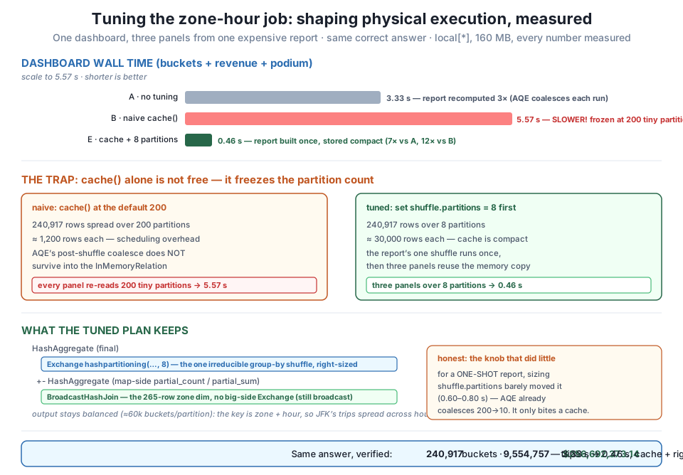
cache() is slower at 5.57 s because it freezes the report at the default 200 shuffle partitions — 240,917 rows spread over 200 near-empty partitions. Setting spark.sql.shuffle.partitions to 8 before caching stores the report compact, and the three panels finish in 0.46 s — about 7× faster than no cache, 12× faster than the naive one. The join stays a BroadcastHashJoin and the output is balanced (no skew: the key is zone + hour). Honest caveat: for a one-shot query the same knob barely moved (0.60–0.80 s) — AQE already coalesces 200 to a handful; it only bites a cache. Answer unchanged: 240,917 buckets, 9,554,757 trips, $256,692,373.14.Why the naive cache lost, in one sentence
AQE right-sizes a shuffle at read time, but cache() stores the shuffle’s written output — so a report that AQE would have run in ~8 coalesced partitions gets frozen into 200 when cached, and every reuse pays 200-partition overhead. Set spark.sql.shuffle.partitions to a sane size before materializing a cache, and the coalescing you’d have gotten for free is baked in instead of lost.
These numbers are from a 160 MB laptop
On one machine over the 160 MB quarter, every absolute time here is small and page-cache-warmed, so treat the ratios as the lesson, not the seconds. The caching win grows with how expensive the shared report is and how many times it’s reused; the partition knob matters more as data grows past the point where even AQE’s coalesced partitions are large. What generalizes is the shape of the reasoning: find the reused expensive node, cache it, and make sure it’s cached at a sane partition count.
Module 4’s project gave you a query-fix checklist — read the plan, kill the UDF, restore the broadcast, prune the read. This project gives you its counterpart: a physical-execution checklist for a job whose logic is already correct but whose runtime you want to shape. When a correct Spark job is slower than it should be, work these in order:
report), never the cheap page-cached Parquet scan under it. Caching a cheap read wastes memory for no gain (Lesson 3).spark.sql.shuffle.partitions to fit the cached result (a handful for hundreds of thousands of rows) before the first action. This is the step that turned the cache from a loss into a 12x win..explain() after tuning: a small dimension must still show BroadcastHashJoin, not a SortMergeJoin with two exchanges. A config change can silently undo a broadcast.spark_partition_id() to count rows per partition. A hot key on the grouping key strands one task; a fine-grained key (zone + hour) usually avoids it. If it doesn’t, revisit Lesson 4’s mitigations.unpersist() when done. A cache you stop needing is memory you stop having.Steps 2 and 3 are the pair most people miss: caching and partition-sizing are not independent knobs on this kind of job — they only work together.
Exercise 1 — Confirm AQE can’t coalesce a cache. Step B blamed the naive cache’s slowness on 200 frozen partitions. Prove the mechanism directly: cache the report at the default 200, print cached.rdd.getNumPartitions(); then set spark.sql.shuffle.partitions to 8, cache a fresh copy, and print its partition count. Show the first is 200 and the second is 8 — the cache stores whatever the shuffle wrote, and AQE’s runtime coalescing never enters.
Hint
Call .cache() then an action (.count()) to materialize before reading .rdd.getNumPartitions() — cache() is lazy, so the count is meaningless until something forces materialization. Change spark.conf.set("spark.sql.shuffle.partitions", "8") before building the second cached report, since the config is read when the Exchange is planned, not when you call cache().
Exercise 2 — Find the partition sweet spot. The tuned job used 8 partitions. Is that best? With the report cached, sweep spark.sql.shuffle.partitions over 1, 4, 8, 16, and 64, materializing a fresh cache for each, and time the full dashboard. Where does it bottom out, and why do very low (under-parallelized) and very high (overhead-heavy) values both hurt?
Hint
You’re re-deriving Lesson 1’s “too few underuses cores, too many adds scheduling overhead” on a cached result. Expect the best time near the core count or a small multiple of it (this machine has 10 cores). At 1 partition the whole dashboard runs single-threaded; at 64 you’re back toward the 200-partition overhead that made the naive cache slow. Remember to unpersist() between settings so caches don’t accumulate.
Exercise 3 — Break the broadcast, then catch it with the checklist. Simulate a config mistake: set spark.sql.autoBroadcastJoinThreshold to -1, rebuild the report, and read .explain(). The join should fall to a SortMergeJoin with two Exchange/Sort pairs. Confirm the answer is still 240,917 buckets and $256,692,373.14 (it’s correct but slower), then restore the broadcast with F.broadcast(zones) or by resetting the threshold, and verify BroadcastHashJoin returns. This is checklist step 4 catching a real regression.
Hint
spark.conf.set("spark.sql.autoBroadcastJoinThreshold", "-1") disables auto-broadcast globally; an explicit F.broadcast(zones) in the join can still force it even then, which is why wrapping the small side is the robust habit. The point is that a correct answer can hide a physical regression — only the plan shows the shuffle you didn’t mean to add.
You took CityFlow’s already-correct zone-hour dashboard and tuned its physical execution without changing a single result. The job forks one expensive report into three panels, so without a cache it recomputes that report three times — 3.33 s of repeated window-filter-join-shuffle work. The obvious fix, a plain cache(), made it slower (5.57 s), because the cache froze the report into the default 200 shuffle partitions and every panel re-read 240,917 rows across 200 near-empty partitions — AQE’s coalescing right-sizes a shuffle at read time but cannot survive into an InMemoryRelation. The real fix coupled two levers: set spark.sql.shuffle.partitions to 8 before caching so the report is stored compact, then cache once. The three panels then finished in about 0.46 s — roughly 7x faster than no tuning and 12x faster than the naive cache — with the join still a BroadcastHashJoin and the output balanced across partitions (no skew, because the grouping key is zone plus hour, scattering even JFK’s trips). Honesty throughout: on a one-shot throwaway query the same partition knob barely moved the time (0.60 to 0.80 s), because AQE already coalesces 200 down to a handful; the knob only earns its keep once you cache. And the tuned job reproduced Course 1 exactly: 240,917 buckets, 9,554,757 trips, $256,692,373.14.
cache() stores the shuffle’s written partitions, and AQE cannot coalesce them afterward, so a cache built at 200 partitions stays slow to reuse.spark.sql.shuffle.partitions does little for a one-shot query (AQE coalesces it) but is decisive for a cached, re-aggregated one; set it to a handful that fits the result..explain() must still show BroadcastHashJoin for a small dimension, never a SortMergeJoin with two exchanges.Real CityFlow jobs arrive correct far more often than they arrive broken, and the request that follows is almost always “make it faster” without “and you may change the answer.” That is exactly this project’s discipline: leave the logic alone, find the reused expensive node, and shape how it runs — cache it, cache it at a sane partition count, keep the small joins broadcast, watch for skew, and verify the answer held every time. The most valuable thing you learned here is that tuning knobs are not independently good: a cache() with the wrong partition count is worse than no cache, and the fix was to use two levers together. That is how physical tuning actually behaves at every scale — the same reasoning that saved a fraction of a second on 160 MB saves hours on the terabyte job that has to finish before the dashboard refreshes at dawn.
You’ve now closed Module 5. Across five lessons you learned to shape Spark’s physical execution rather than rewrite its logic: what a partition is and how many the data lands in, the shuffle that moves rows between them, when caching a reused result pays and when it quietly costs, how a hot key strands one task, and — in this project — how to pull all of it together on one job, measuring every change and verifying the answer never drifted from Course 1’s ground truth. The through-line of the whole module was that performance lives in how the work runs on the machine, not just what the query says. Module 6, Building ETL Pipelines in Spark, changes the question again: from tuning a single analytical job to composing many stages into a dependable pipeline — reading from sources, transforming through well-defined steps, writing partitioned output, and handling the failures and re-runs that a one-off script never has to survive. The zone-hour report you have now written, read, optimized, and tuned becomes one stage in something larger, and everything you learned about partitions, shuffles, caching, and skew is what will keep that pipeline fast when it runs every night instead of once.
Keep DATATWEETS free. Help fund practical data, AI, and engineering lessons for learners worldwide.
