Title here
Summary here
Module 1 left CityFlow with a debt. Twice, something strange happened on screen and was deferred with a promise: reading all three monthly files — 160.4 MB, 9,554,778 rows — “finished” in 59 ms, while a mere count() of the same data took real, visible time. A pandas engineer’s cost model runs exactly backwards from that: reading is the expensive part you wait for, and counting something already in memory is free. Spark inverted the ledger, Module 1 said “that’s lazy evaluation, Module 2 owns it,” and moved on. This is Module 2. The bill is due.
The explanation is one sentence — transformations build a plan; actions execute it — but a sentence is not a mental model, so this lesson makes you feel the split with a stopwatch. You will rebuild Module 1’s mystery moment, timed. Then you will build something much bigger: the full zone-hour report pipeline from Course 1 — window filter, hour truncation, group by zone and hour, trip count and revenue sum over 9,554,778 rows — and watch all of it “complete” in 73 ms, because nothing completed at all. explain() will show you the plan Spark wrote instead of working. Then one action executes that plan in 2.31 s, and the numbers that come back — 240,917 buckets, 9,554,757 trips, $256,692,373.14 — match Course 1’s verified report to the cent. And then the trap this lesson exists to spare you from: ask the same lazy DataFrame two questions, and Spark runs the entire pipeline twice. We’ll measure that, explain why it must be so, and name — without teaching — the fix that Module 5 owns.
By the end of this lesson, you will be able to:
explain() to prove a plan exists before any work happens, and find the scan and the filter inside itYou’ll need pyspark with the JDK configured as in Module 1, Lesson 3 — nothing else today. Start the session.
Same session shape as always — named, local, quiet:
import warnings
warnings.filterwarnings("ignore")
import time

from pyspark.sql import SparkSession

spark = (SparkSession.builder
         .appName("cityflow")
         .master("local[*]")
         .config("spark.ui.showConsoleProgress", "false")
         .getOrCreate())
spark.sparkContext.setLogLevel("ERROR")
print("Spark", spark.version, "-", spark.sparkContext.defaultParallelism, "task slots")
Spark 4.2.0 - 10 task slotsNow reproduce Module 1’s strange moment deliberately, with the stopwatch running on both halves. One detail made explicit this time: Lesson 3 measured that the very first read of a session carries about a second of one-time warmup while the JVM loads its I/O machinery, so we spend that warmup on an untimed throwaway read first. What we’re timing is the read itself, not the engine waking up:
months = ["yellow_tripdata_2024-01.parquet",
          "yellow_tripdata_2024-02.parquet",
          "yellow_tripdata_2024-03.parquet"]

spark.read.parquet(*months)   # untimed warm-up: first touch loads the JVM's I/O machinery

t0 = time.perf_counter()
trips = spark.read.parquet(*months)
read_ms = (time.perf_counter() - t0) * 1000
print(f"'read' three files, 160.4 MB: {read_ms:.0f} ms")

t0 = time.perf_counter()
n_rows = trips.count()
count_secs = time.perf_counter() - t0
print(f"count() -> {n_rows:,} rows: {count_secs:.2f} s")
'read' three files, 160.4 MB: 69 ms
count() -> 9,554,778 rows: 1.00 sThere it is again, in one screen: “reading” 160.4 MB took 69 ms, and counting what was “already read” took a full second — fourteen times longer. The count is right, of course: 9,554,778 is the quarter total Course 1 verified and Module 1 re-verified. But the shape of the timing is upside down by every pandas instinct, and this time we don’t defer. Here is the whole explanation, and the rest of the lesson is evidence for it:
spark.read.parquet is not a read. It is a promise of a read. It opened three file footers, noted the schema and row-group layout, and returned a DataFrame that contains no rows — a DataFrame in Spark is a plan, a description of how to produce data, not the data. Work happened only when count() demanded an answer, because an answer cannot be described — it has to be computed. Calls that extend the plan are transformations. Calls that demand an answer are actions. Every timing oddity you will ever see in Spark starts with knowing which one you just typed.
If a read is just a plan entry, the natural question is how far you can push the plan before anything runs. The answer: arbitrarily far. So let’s push it somewhere real — the flagship artifact of Course 1, CityFlow’s zone-hour report: for every pickup zone and every clock hour of the quarter, how many trips and how much revenue? Course 1 built it with chunked pandas and verified it to the cent; you’re about to express the same report in four calls.
The logic, in order: keep only pickups inside the quarter window (January 1 up to but not including April 1 — Course 1’s window, the one that quarantines the 21 stray-timestamp rows with pickup times in 2002 and 2009); truncate each pickup to its hour; group by zone and hour; count trips and sum revenue per group. Timed:
from pyspark.sql import functions as F

t0 = time.perf_counter()
report = (trips
          .filter((F.col("tpep_pickup_datetime") >= "2024-01-01") &
                  (F.col("tpep_pickup_datetime") < "2024-04-01"))
          .withColumn("hour", F.date_trunc("hour", F.col("tpep_pickup_datetime")))
          .groupBy("PULocationID", "hour")
          .agg(F.count("*").alias("trips"),
               F.sum("total_amount").alias("revenue")))
build_ms = (time.perf_counter() - t0) * 1000

print(f"four transformations over 9,554,778 rows: {build_ms:.0f} ms")
print(f"report is a {type(report).__name__} - and Spark has not touched a single row")
four transformations over 9,554,778 rows: 73 ms
report is a DataFrame - and Spark has not touched a single rowRead that top line the way a pandas user would have to: a filter over 9.5 million timestamps, a derived column on every surviving row, a group-by producing hundreds of thousands of groups, two aggregates per group — 73 milliseconds, total. In pandas, every one of those lines executes as you type it; the groupby alone on this quarter is seconds of real work and, before that, the quarter has to exist in memory — all ~1,347 MB of it. Spark did none of that. Each call took report’s plan, appended one step, and returned a new DataFrame wrapping the longer plan. (Why a new one — why Spark never modifies a DataFrame in place — is Lesson 4’s subject, and the payoff for it is Spark’s whole fault-tolerance story.)
It’s worth being precise about what those 73 ms did buy, because “lazy” doesn’t mean “nothing happened.” Spark analyzed each call: it checked that tpep_pickup_datetime, PULocationID, and total_amount exist and have types the operations accept — misspell a column here and you get an error immediately, laziness notwithstanding. What it did not do is read, filter, truncate, group, or sum one single row. report is a recipe for the zone-hour report. The report itself does not exist anywhere.
That claim — “the plan exists, the work doesn’t” — sounds like something you have to take on faith. You don’t. Spark will show you the plan.
Every DataFrame carries its plan, and explain() prints the physical version of it — what Spark intends to do the moment an action forces its hand:
report.explain()== Physical Plan ==
AdaptiveSparkPlan isFinalPlan=false
+- HashAggregate(keys=[PULocationID#26, hour#62], functions=[count(1), sum(total_amount#35)])
+- Exchange hashpartitioning(PULocationID#26, hour#62, 200), ENSURE_REQUIREMENTS, [plan_id=51]
+- HashAggregate(keys=[PULocationID#26, hour#62], functions=[partial_count(1), partial_sum(total_amount#35)])
+- Project [PULocationID#26, total_amount#35, date_trunc(hour, cast(tpep_pickup_datetime#20 as timestamp), Some(Asia/Tehran)) AS hour#62]
+- Filter ((isnotnull(tpep_pickup_datetime#20) AND (tpep_pickup_datetime#20 >= 2024-01-01 00:00:00)) AND (tpep_pickup_datetime#20 < 2024-04-01 00:00:00))
+- FileScan parquet [tpep_pickup_datetime#20,PULocationID#26,total_amount#35] Batched: true, DataFilters: [isnotnull(tpep_pickup_datetime#20), (tpep_pickup_datetime#20 >= 2024-01-01 00:00:00), (tpep_pick..., Format: Parquet, Location: InMemoryFileIndex(3 paths)[...], PartitionFilters: [], PushedFilters: [IsNotNull(tpep_pickup_datetime), GreaterThanOrEqual(tpep_pickup_datetime,2024-01-01T00:00), Less..., ReadSchema: struct<tpep_pickup_datetime:timestamp_ntz,PULocationID:int,total_amount:double>(Output shown verbatim except the Location: file paths, shortened to [...] — yours will show your own directory.)
Module 4 teaches you to read plans like this line by line; today we take exactly three observations from it, bottom-up, because plans read from the bottom (first thing done) to the top (last):
Find the scan. The bottom line, FileScan parquet, is the read — 3 paths, our three monthly files. Look at its ReadSchema: tpep_pickup_datetime, PULocationID, total_amount. Three columns. The files have nineteen, and nobody wrote a select — Spark noticed on its own that the plan only ever uses three columns and pruned the other sixteen out of the scan. This is the payoff of laziness in one detail: because Spark waited until it could see the whole program, its optimizer could rewrite the beginning of the program in light of the end. An eager engine that executes line by line never gets that chance — by the time pandas knows you only needed three columns, it has already materialized nineteen.
Find the filter. One level up, Filter holds our window condition — and notice the scan below it also lists our dates under PushedFilters, meaning Spark handed the condition to the Parquet reader itself to skip data early where it can. Same lesson: whole-plan visibility turns your line order into its preferred order. (One honest footnote: Course 1 measured that these particular files ship without row-group statistics, so pushdown has little to prune against here — the mechanism is real, the savings on these files modest.)
Find the plan-about-the-plan. The very top line says AdaptiveSparkPlan isFinalPlan=false. That is AQE — adaptive query execution, on by default in Spark 4: Spark reserves the right to re-plan mid-flight using statistics it gathers as it runs (you met this in Module 1 when one action showed up as two jobs with skipped stages). isFinalPlan=false means even this printed plan is provisional. Module 4 goes deep; for today, the word to keep is the one this whole lesson is about: plan. It exists, it’s inspectable, and printing it launched zero jobs — check the Spark UI at localhost:4040 right now and the Jobs page is still empty of any aggregation work.
Why does my plan mention a time zone?
Inside the Project line you can see date_trunc(hour, cast(... as timestamp), Some(Asia/Tehran)) — this machine’s session time zone; yours will show yours. The pickup column is timestamp_ntz (no time zone, as Module 1 established), and date_trunc casts it through the session zone to do calendar math. Because the same zone is used to interpret and to display, the hour buckets land on the data’s own wall-clock hours regardless of what your session zone is — which is why the bucket count below matches Course 1 exactly. The general reflex is Course 1’s: whenever timestamps cross a representation boundary, stop and check the units and the zone.
The plan exists; the report doesn’t. Ask for an answer — how many zone-hour buckets does the quarter have? — and Spark finally has to execute:
t0 = time.perf_counter()
n_buckets = report.count()
action_secs = time.perf_counter() - t0
print(f"count() -> {n_buckets:,} zone-hour buckets in {action_secs:.2f} s")
count() -> 240,917 zone-hour buckets in 2.31 sTwo things on that line, and both matter.
First, the number: 240,917. That is exactly the bucket count of Course 1’s zone-hour report — built there by a chunked pandas pipeline, verified against the quarter’s revenue to the cent, trusted by CityFlow ever since. Spark expressed the same report in four calls and reached the identical shape on the first try. The cross-verification habit from Module 1 carries forward: a new engine earns trust by matching the audited one.
Second, the time: 2.31 s, against 73 ms to build the plan — a 32× gap between describing the work and doing it. Now the whole pipeline actually ran: ten task slots scanned 160.4 MB across the three files, decoded three columns, filtered 9,554,778 timestamps down to 9,554,757, truncated every survivor to its hour, hash-aggregated them into 240,917 groups — twice, in fact: once partially within each partition and once finally after the Exchange regrouped them, exactly as the plan’s two HashAggregate lines promised. (That Exchange — the shuffle — is a cost center important enough to get all of Module 5. Today it’s just a line you can now recognize.)
This is the honest reading of every “Spark is instant” demo you will ever see: an instant return is a transformation, and it proves nothing about cost. The cost shows up at the action — all of it.
Here is the moment this lesson has been building toward, and the single most common performance surprise in real Spark code. report.count() just computed the full report. Surely asking the same question again is free — the work is done, the engine must remember?
t0 = time.perf_counter()
n_again = report.count()
again_secs = time.perf_counter() - t0
print(f"the same count() -> {n_again:,} buckets in {again_secs:.2f} s")
the same count() -> 240,917 buckets in 0.79 s0.79 seconds. Not milliseconds — not the 73 ms a plan costs. Spark re-ran the entire pipeline: re-scanned all three files, re-filtered 9.5 million rows, re-built all 240,917 groups, and only then re-answered a question it had answered seconds earlier. Honesty about the number: the second run is faster than the first — 0.79 s against 2.31 s — but not because Spark kept anything. The operating system kept the file bytes in its page cache, and the JVM reuses the query code it compiled for run 1; the pipeline itself executed again, end to end. Open the Spark UI and you’ll see it plainly: a second, separate job with its own full set of stages and tasks.
Why must it be this way? Because a DataFrame is a plan, and executing a plan produces the answer — not a stored copy of the data along the way. The 240,917 result of run 1 was handed to Python as an integer and forgotten; the 9,554,757 filtered-and-grouped rows it passed through existed only transiently, partition by partition, and were released as each task finished. That frugality is a feature — it is exactly why Module 1’s quarter never needed 1,347 MB of memory the way pandas did — but it has this price: nothing is materialized unless you instruct Spark to materialize it. There is an instruction for that — cache() — and it belongs to Module 5, where its costs get measured as honestly as its benefits. Today, know the trap exists and know how to spot it: any lazy DataFrame that gets more than one action re-executes its full plan for each one.
And it’s not just repeated questions — any action pays full price. Ask the report for its totals, which is also our deepest cross-check of the day:
t0 = time.perf_counter()
totals = report.agg(F.sum("trips").alias("trips"),
                    F.sum("revenue").alias("revenue")).first()
totals_secs = time.perf_counter() - t0
print(f"{totals['trips']:,} trips, ${totals['revenue']:,.2f} in {totals_secs:.2f} s")
9,554,757 trips, $256,692,373.14 in 1.16 sA third full execution — 1.16 s — and a handshake across two engines and two courses: 9,554,757 trips kept (the quarter’s 9,554,778 rows minus the 21 stray-timestamp quarantines) and $256,692,373.14 total revenue, matching Course 1’s verified report to the cent. Note what carrying the cent implies: Course 1 established that ~31,000 repeated trip keys per month are fare reversals whose positive and negative amounts must both stay in the data for SUM to cancel them. Spark’s sum landing on the exact same cent means those reversals flowed through this pipeline intact too.
One more action, because the report deserves to be seen — its busiest buckets:
t0 = time.perf_counter()
report.orderBy(F.col("trips").desc()).show(5)
show_secs = time.perf_counter() - t0
print(f"orderBy + show(5): {show_secs:.2f} s - a fourth full run")
+------------+-------------------+-----+------------------+
|PULocationID| hour|trips| revenue|
+------------+-------------------+-----+------------------+
| 79|2024-02-25 01:00:00| 846|17891.310000000027|
| 79|2024-02-25 00:00:00| 803|17371.510000000006|
| 161|2024-02-29 17:00:00| 779| 20840.14000000002|
| 79|2024-03-09 01:00:00| 762|15905.109999999993|
| 79|2024-02-25 02:00:00| 727|15024.619999999977|
+------------+-------------------+-----+------------------+
only showing top 5 rows
orderBy + show(5): 0.98 s - a fourth full runFour answers, four executions: 2.31 s + 0.79 s + 1.16 s + 0.98 s of repeated work on one unchanging pipeline. (The exact seconds wobble run to run with machine load; the pattern — every action a full run — is the invariant.) The rows themselves are a small CityFlow reward: the quarter’s single busiest zone-hour is zone 79 — East Village — at 1 a.m. on Sunday, February 25, 846 pickups in one hour, with midnight and 2 a.m. that same night in the top five: bar close, captured in a group-by. The one non-nightlife entry is zone 161, Midtown Center, at 5 p.m. on leap day — a Thursday rush hour. And those ragged revenue decimals (17891.310000000027) are Module 1’s honest footnote resurfacing: money stored as double accumulates floating-point dust; a later module deals with it properly.
Notebooks make this trap almost invisible
In a notebook, the twice-run trap rarely looks like two count() calls in a row. It looks like a show() here to eyeball the data, a count() two cells later for a sanity check, a toPandas() at the bottom for a chart — three innocent cells, three full executions of every transformation above them. When a “fast” notebook turns slow as it grows, count the actions before you blame the data size. The Spark UI’s Jobs page is the audit trail: every line there is a full trip through your plan.
You now have the working test: does this call require Spark to produce an answer? If the result is another DataFrame — a longer plan — it’s a transformation and will return in milliseconds no matter the data size. If the result is a number, rows, a file on disk, or anything Python can hold, it’s an action and costs a full execution. The table below is the vocabulary you’ll use all course; notice it’s the return type that gives each row away:
| Call | Kind | What actually happens |
|---|---|---|
select, filter / where, withColumn, drop | transformation | plan grows; returns a new DataFrame |
groupBy(...).agg(...), join, union, distinct | transformation | plan grows — even the “heavy” ones |
orderBy / sort, limit | transformation | still just the plan; limit does not fetch rows |
count(), collect(), take(n), first() | action | executes the plan; result lands in Python |
show(n) | action | executes enough of the plan to print n rows |
write.parquet(...) and friends | action | executes the plan; result lands on disk |
toPandas() | action | executes the plan and ships everything to the driver — Module 1’s crash lives here |
printSchema(), columns, explain() | neither | reads plan metadata; no job at all |
Three of those rows repay a second look. limit(5) and take(5) sound like synonyms and are on opposite sides of the divide: limit is a transformation (a plan step meaning “at most 5 rows survive this point”), while take is the action that actually goes and gets 5 rows. write being an action surprises people who think of actions as “small results” — the definition is not small, it’s demanded: writing files demands execution just as surely as counting does. And the bottom row is why you could printSchema() and explain() all day in Module 1 without ever launching a job — schema and plan are metadata Spark already holds; no rows are needed to show them.
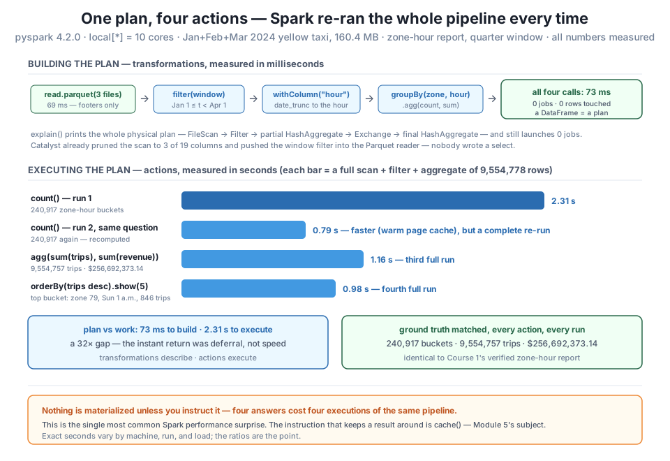
filter → withColumn → groupBy → agg over 9,554,778 rows) took 73 ms and launched zero jobs; explain() printed the complete physical plan — scan pruned to 3 of 19 columns, filter pushed into the reader — still without touching a row. Then every action paid full price: count() executed the pipeline in 2.31 s (240,917 buckets), the identical count() re-executed everything in 0.79 s (faster only because the OS page cache was warm), the totals action ran it a third time (9,554,757 trips · $256,692,373.14 — Course 1's report to the cent), and show(5) a fourth. Nothing is materialized unless you instruct it; the instruction is Module 5's cache(). Exact seconds vary run to run; the 32× plan-versus-work ratio is the point.The session’s work is done — release it:
spark.stop()
print("session stopped")
session stoppedExercise 1 — Predict the bill, then run it. Before executing anything, write down how many Spark jobs this sequence launches: read the three months; select pickup time and total_amount; filter to the quarter window; limit(10); take(10); count() on the un-limited filtered frame; printSchema(). Then run it with time.perf_counter() around each line and check your prediction against both the timings and the Spark UI’s Jobs page.
Hint
Score it with the return-type test. read, select, filter, and limit all hand back DataFrames — plan only, milliseconds each. take(10) is an action (it’s limit’s eager twin), count() is an action, and printSchema() is neither — metadata, no job. So: two answers demanded, at least two jobs (AQE may split one action into more — count what the UI actually shows and don’t be alarmed if it’s not exactly two). If your limit(10) line took milliseconds while take(10) took real time, you’ve caught the pair red-handed.
Exercise 2 — The trap at JFK. Module 1, Lesson 3 counted JFK’s windowed pickups: 429,745. Rebuild that lazily — filter the quarter to PULocationID == 132 inside the window — and then, timing each: call .count(), call .count() again, and call .show(3). How many times did Spark scan the three files? Confirm your answer on the Spark UI’s Jobs page, and write one sentence predicting what would change if a cache() sat after the filter (you’ll verify that prediction in Module 5).
Hint
Both counts must return exactly 429,745 — if you get 429,746, your window is missing and you’ve re-found Module 1’s stray-timestamp trip; the files and the quarter are different populations. Expect three actions, three full executions: comparable real time each (the first usually slowest — cold caches), never the milliseconds a mere transformation would cost. The one-sentence prediction: with a cache, run 1 would pay to build and store the filtered rows, and runs 2-3 would read the stored copy instead of the files — cost moves from every-action to once.
Exercise 3 — Read a second plan. Build the simplest useful pipeline — trips.groupBy("PULocationID").count() with no filter and no extra columns — and call explain() on it before any action. In the FileScan line, how many columns does ReadSchema list this time? Compare with the lesson’s plan (3 of 19) and explain the difference in one sentence. Then run .count() on it and check the resulting number of zones against what you know from Module 1’s aggregations.
Hint
Your pipeline touches exactly one column, so ReadSchema should list PULocationID alone — 1 of 19, pruned even harder than the lesson’s plan, because Catalyst prunes to whatever the whole visible program needs and nothing more. The zone count to expect: Module 1’s windowed aggregation found 262 distinct pickup zones; without the window filter your count may differ by a zone or two if any stray-timestamp row hides in an otherwise-absent zone — a difference worth checking rather than assuming.
Module 1’s deferred mystery is closed. Reading 160.4 MB “finished” in 69 ms because spark.read.parquet is a transformation — it promises a read and returns a plan — while count() is an action that executed the plan and took a real 1.00 s to confirm all 9,554,778 rows. Building Course 1’s entire zone-hour report as a pipeline — window filter, date_trunc to the hour, groupBy zone and hour, count plus revenue sum — took 73 ms and launched zero jobs; explain() printed the complete physical plan before any work existed, with Catalyst already pruning the scan to 3 of 19 columns and pushing the window filter into the Parquet reader, unasked, plus an AdaptiveSparkPlan isFinalPlan=false header announcing that AQE may still re-plan at runtime. The first action paid the full bill: 2.31 s — a 32× gap over plan-building — returning 240,917 zone-hour buckets, exactly Course 1’s verified count. Then the trap, measured: the identical count() re-executed the entire pipeline in 0.79 s (faster only via the OS page cache — the Spark UI shows a complete second job), a totals action ran everything a third time (9,554,757 trips, $256,692,373.14 — Course 1’s report to the cent, fare reversals intact), and show(5) a fourth, surfacing East Village at 1 a.m. Sunday as the quarter’s busiest zone-hour (846 trips). Nothing is materialized unless you instruct it; the instruction — cache() — and its real costs belong to Module 5.
select, filter, withColumn, groupBy().agg(), join, orderBy, limit. It appends to the plan and returns in milliseconds at any data size — 73 ms for four of them over 9.5M rows.count, collect, take, first, show, write, toPandas. Only actions launch jobs; each one executes the full plan — 2.31 s for the same pipeline the transformations “finished” in 73 ms.cache()) is Module 5’s, costs included.explain() — prints the physical plan without running anything: read it bottom-up (scan first), find FileScan’s ReadSchema and PushedFilters, and recognize AdaptiveSparkPlan isFinalPlan=false as Spark 4’s AQE reserving the right to re-plan — Module 4 reads plans in full.CityFlow’s engineers are about to write Spark pipelines dozens of transformations long, and every scheduling decision, every code review comment, every “why is this slow” investigation in that future starts with the distinction this lesson measured. An engineer who can’t tell transformations from actions reads Spark timings backwards — they’ll benchmark the 73 ms plan-build and report a miracle, or watch a notebook re-scan a quarter of data five times for five casual show() calls and blame the cluster. The twice-run trap in particular is not a beginner’s stumble; it is the recurring performance bug in production Spark code, because it hides so well — each individual action looks innocent, and the waste only shows up as a pipeline that gets mysteriously slower as colleagues append cells to it. You now have the audit method: count the actions, check the Jobs page, know that every answer re-runs the plan. And you have the deeper trade to weigh: Spark’s refusal to materialize anything is the same frugality that let this quarter aggregate without pandas’ 1,347 MB footprint — laziness giveth exactly where it taketh. Knowing when to override that refusal — when storing beats recomputing — is a genuine engineering judgment, and it gets its own module because judgments deserve measurements.
You’ve now seen the lazy bargain from above — the API where four calls build a plan and one call executes it. Lesson 2, RDDs Underneath, takes you below the DataFrame to the layer everything compiles down to: the RDD, Spark’s raw distributed collection, where there is no optimizer, no column pruning, no pushed filters — just your Python functions applied to raw rows. You’ll take the zone-count job you just expressed in DataFrame calls and hand-roll it with map and reduceByKey lambdas, then measure the gap — and it is not subtle, because every lambda drags rows across the JVM-to-Python boundary and Catalyst can’t optimize code it can’t see into. The plan you learned to print today is exactly what the RDD version doesn’t get, and putting the two side by side is the fastest way to understand what the DataFrame API has quietly been doing for you — and when dropping down to RDDs is still the right call.
Keep DATATWEETS free. Help fund practical data, AI, and engineering lessons for learners worldwide.
