Lesson 2 - RDDs Underneath

Welcome to RDDs Underneath#

Lesson 1 established the rule this module runs on: transformations build a plan, actions execute it, and the gap between those two moments is where Spark hides everything interesting. But “Spark builds a plan” raises an obvious question that lesson deliberately left open — a plan of what? When the optimizer finishes rearranging your groupBy, something concrete has to actually run on ten cores. That something is the RDD — the Resilient Distributed Dataset, Spark’s original API, the thing the 2011 research project was before DataFrames existed, and still the substrate every DataFrame operation compiles down to. It has never gone away. It is one attribute access away: df.rdd.

CityFlow’s engineers will rarely choose to write RDD code, and this lesson is honest about why — but “rarely” is not “never,” and more importantly, you cannot reason about what the DataFrame API is doing for you until you have felt what life is like without it. So today you drop one level down. You’ll meet the RDD under the January DataFrame and see what a Row actually is, drive RDDs directly with map, filter, and reduceByKey using plain Python lambdas on real trips, and then run the race this lesson exists for: the per-zone trip count — whose January answer Course 1 pinned exactly — hand-rolled on RDDs versus written against the DataFrame API, on the same file, same session, same measurement policy. The gap is 51.4x, it is not folklore, and by the end you’ll be able to point at the exact two mechanisms that cause it in the plans Spark prints.

By the end of this lesson, you will be able to:

• Define an RDD — resilient, distributed, dataset — and expose the one underneath any DataFrame with df.rdd
• Drive RDDs directly with map, filter, and reduceByKey, passing plain Python lambdas over real trip data
• Measure what hand-rolling costs — 7.93 s vs 0.15 s (51.4x) for the same zone count — and attribute it to the JVM→Python bridge and a blinded optimizer
• Read the evidence in two plans: a pruned ReadSchema with partial aggregation vs opaque PythonRDD stages in toDebugString
• Name the few situations where dropping to the RDD level is still the right engineering call

You’ll need pyspark only — everything in this lesson happens inside Spark itself.

Resilient Distributed Dataset — Three Words, Each Load-Bearing#

One paragraph of history, because it explains why this layer exists and why you’ll mostly see it through a porthole. RDDs were Spark: the original UC Berkeley research (2011, formalized in a 2012 paper) proposed the RDD as the core abstraction — an immutable, partitioned collection of arbitrary objects, each partition recomputable from its lineage if a machine dies. Every early Spark program was map and reduceByKey on RDDs. DataFrames arrived in 2015 with the Catalyst optimizer attached, and the pitch was exactly the trade this lesson measures: describe what you want in a structured API, and an optimizer — not you — decides how to run it. DataFrames won so completely that the RDD API has been in maintenance mode for years. But it never disappeared, because it couldn’t: DataFrame plans still compile to RDD operations. It’s the assembly language under the compiler.

Each word in the name is a design decision. Dataset: a collection of arbitrary objects — not columns, not a schema, just objects, which is why Python lambdas can do anything to them. Distributed: the collection is split into partitions that live (on a real cluster) on different machines and are processed in parallel — the same partitions Module 1 counted. Resilient: each RDD remembers the operations that produced it from its parent, so a lost partition can be recomputed instead of restored from a copy — that lineage story is Lesson 4’s whole subject. For now, let’s simply look at one. Standard session, January file:

import warnings
warnings.filterwarnings("ignore")
import time
import statistics

from pyspark.sql import SparkSession

spark = (SparkSession.builder
         .appName("cityflow")
         .master("local[*]")
         .config("spark.ui.showConsoleProgress", "false")
         .getOrCreate())
spark.sparkContext.setLogLevel("ERROR")
sc = spark.sparkContext

df = spark.read.parquet("yellow_tripdata_2024-01.parquet")
print(type(df.rdd))
print("partitions:", df.rdd.getNumPartitions())

<class 'pyspark.core.rdd.RDD'>
partitions: 10

No conversion function, no export — the RDD is just there, and it reports the same 10 partitions Module 1 measured for a January read on this machine (plan follows cores; local[*] is 10 here). Note we also grabbed sc, the SparkContext — the older, lower-level handle that RDD-era code is written against. The SparkSession you’ve used all course wraps it; every session carries one.

So what’s in this collection? At DataFrame level, January is columns and a schema. At RDD level, it’s 2,964,624 Python objects — and it’s worth looking one in the eye:

row = df.rdd.first()
print(row)
print()
print("row['PULocationID'] =", row["PULocationID"])
print("row.trip_distance   =", row.trip_distance)

Row(VendorID=2, tpep_pickup_datetime=datetime.datetime(2024, 1, 1, 0, 57, 55), tpep_dropoff_datetime=datetime.datetime(2024, 1, 1, 1, 17, 43), passenger_count=1, trip_distance=1.72, RatecodeID=1, store_and_fwd_flag='N', PULocationID=186, DOLocationID=79, payment_type=2, fare_amount=17.7, extra=1.0, mta_tax=0.5, tip_amount=0.0, tolls_amount=0.0, improvement_surcharge=1.0, total_amount=22.7, congestion_surcharge=2.5, Airport_fee=0.0)

row['PULocationID'] = 186
row.trip_distance   = 1.72

A Row is a real Python object — tuple-like, with fields accessible by key or by attribute, timestamps already materialized as datetime.datetime values. That’s genuinely convenient: your lambdas get to treat trips like ordinary Python data. Hold on to the uncomfortable half of that convenience, though. This object had to be built — the trip’s bytes serialized out of the JVM, shipped to a Python process, and assembled into a Row — and at RDD level that happens for every row you touch. One row, charming. 2,964,624 of them is a bill, and we’re about to get it itemized.

RDDs Speak Raw Python#

The RDD API is the functional-programming trio — map transforms each element, filter keeps some, reduce/reduceByKey combines them — and its superpower is that the elements can be anything. No schema required, no columns declared. The cleanest way to feel that is data that genuinely has no schema yet: a raw text file. CityFlow’s zone lookup (taxi_zone_lookup.csv, 265 zones, plain unquoted CSV) makes a perfect small target — read it as bare lines with sc.textFile and impose structure ourselves, one lambda at a time:

lines = sc.textFile("taxi_zone_lookup.csv")
header = lines.first()
zone_names = (lines.filter(lambda line: line != header)
                   .map(lambda line: line.split(","))
                   .map(lambda parts: (int(parts[0]), parts[2]))
                   .collectAsMap())
print(f"parsed {len(zone_names)} zones")
print("132 ->", zone_names[132], "| 161 ->", zone_names[161], "| 237 ->", zone_names[237])

parsed 265 zones
132 -> JFK Airport | 161 -> Midtown Center | 237 -> Upper East Side South

Read the chain like a story: keep every line that isn’t the header, split each survivor on commas, keep fields 0 and 2 as an (id, name) pair, and collectAsMap() the pairs into a Python dict. Notice two things. First, Lesson 1’s law holds down here unchanged — filter and map returned instantly because they’re transformations building a plan; only collectAsMap() (an action) ran anything. Laziness isn’t a DataFrame feature; it’s an RDD feature that DataFrames inherited. Second, this is the RDD API in its natural habitat: schemaless input, arbitrary Python logic, small data. We’ll keep this dict — it names the winners later. (One caveat before you reuse the trick in anger: split(",") only works because this particular file has no quoted commas. A real CSV parser exists for a reason.)

The Same Trick Meets Three Million Rows#

Now point the same elegant API at the trips themselves. Course 1 established January’s busiest pickup zone: JFK Airport, 145,240 trips. Here is that count as an RDD filter with a lambda, and — same session, same warmed file — as a DataFrame where. One timed run each; with the gap you’re about to see, run-to-run jitter is beside the point (the headline race below uses the full warm-up-and-median policy):

df.count()  # warm the OS page cache before any timing

t0 = time.perf_counter()
jfk_rdd = df.rdd.filter(lambda row: row["PULocationID"] == 132).count()
rdd_secs = time.perf_counter() - t0

t0 = time.perf_counter()
jfk_frame = df.where(df.PULocationID == 132).count()
frame_secs = time.perf_counter() - t0

print(f"RDD filter : {jfk_rdd:,} JFK pickups in {rdd_secs:5.2f} s")
print(f"DataFrame  : {jfk_frame:,} JFK pickups in {frame_secs:5.2f} s")
print(f"same answer: {jfk_rdd == jfk_frame}   gap: {rdd_secs/frame_secs:.0f}x")

RDD filter : 145,240 JFK pickups in  7.74 s
DataFrame  : 145,240 JFK pickups in  0.25 s
same answer: True   gap: 31x

Both engines land on 145,240 — Course 1’s number, to the trip. Correctness is not the issue and never will be in this lesson. The issue is that the lambda version took 7.74 seconds against 0.25 — a 31x gap on the most innocent-looking one-liner in the API. Think about what row["PULocationID"] == 132 requires: to evaluate a Python expression, every one of 2,964,624 trips must become a Python Row object first — all nineteen fields of it, datetime conversions included — because Spark cannot know your lambda only needed one column. The DataFrame version never left the JVM: df.PULocationID == 132 isn’t Python logic, it’s a description that Catalyst compiled into a comparison over one column of Parquet. Same question, but one version phrased it where the optimizer could read it.

The Race: Hand-Rolled RDD vs Catalyst#

Time to run the real experiment properly. The job: trips per pickup zone for January — the classic map-to-pairs-then-reduceByKey pattern that was idiomatic Spark for the API’s first four years, versus the one-line DataFrame groupBy. Three implementations: the DataFrame API; the naive hand-rolled RDD over full rows; and a hybrid where we manually select the one needed column before dropping to the RDD — doing Catalyst’s column pruning ourselves, by hand, to see how much of the gap is I/O and how much is something deeper. Measurement policy as always in this course: one untimed warm-up call, then the median of three timed runs.

A word on size, since honesty about method is the course’s habit: this race runs on one month, deliberately. Per-row Python over the full 9.5M-row quarter would cost this lesson several minutes per measurement pass for no additional insight — the per-row toll scales with rows, so the quarter would roughly triple the RDD times (about 25 s a pass) while the DataFrame stayed under a second. One month shows the mechanism at a price we can afford to measure four times per contender.

def bench(fn):
    """One untimed warm-up call, then the median of three timed calls."""
    fn()
    runs = []
    for _ in range(3):
        t0 = time.perf_counter()
        result = fn()
        runs.append(time.perf_counter() - t0)
    return statistics.median(runs), result

def zone_counts_rdd():
    return (df.rdd
            .map(lambda row: (row["PULocationID"], 1))
            .reduceByKey(lambda a, b: a + b)
            .collect())

def zone_counts_rdd_pruned():
    return (df.select("PULocationID").rdd
            .map(lambda row: (row[0], 1))
            .reduceByKey(lambda a, b: a + b)
            .collect())

def zone_counts_frame():
    return df.groupBy("PULocationID").count().collect()

t_frame, res_frame = bench(zone_counts_frame)
t_pruned, res_pruned = bench(zone_counts_rdd_pruned)
t_rdd, res_rdd = bench(zone_counts_rdd)

print(f"DataFrame groupBy     : {t_frame:5.2f} s")
print(f"RDD, pruned by hand   : {t_pruned:5.2f} s   ({t_pruned/t_frame:4.1f}x slower)")
print(f"RDD, full rows        : {t_rdd:5.2f} s   ({t_rdd/t_frame:4.1f}x slower)")

DataFrame groupBy     :  0.15 s
RDD, pruned by hand   :  2.02 s   (13.1x slower)
RDD, full rows        :  7.93 s   (51.4x slower)

(The first reduceByKey may print a stderr suggestion to install psutil for shuffle-spill accounting — harmless for a job this small, and trimmed from the outputs here.)

Three lines, and the whole argument is in the spacing between them. The DataFrame does the job in 0.15 seconds. The idiomatic 2013-style RDD version takes 7.93 seconds — 51.4x slower — and across repeated sessions on this machine that multiple wobbled between roughly 51x and 59x (the denominator is only 0.15 s), so read it as “fifty-ish times,” not a constant of nature. The middle line is the diagnostic gem: hand-pruning to one column before dropping down recovers a huge chunk (7.93 → 2.02 s), which tells you most of the naive version’s pain was reading and shipping nineteen columns when the lambda needed one — the exact optimization Catalyst applies without being asked. But the pruned version is still 13.1x slower, and that residue is the part no amount of hand-tuning removes: the rows themselves still cross into Python one at a time.

Speed means nothing if the answers drift, so: do all three implementations agree, and do they match what Course 1 established? January’s podium, with names courtesy of the zone dict our own RDD built earlier:

as_pairs = sorted((r["PULocationID"], r["count"]) for r in res_frame)
print("all three agree:", as_pairs == sorted(res_rdd) == sorted(res_pruned))
for zone_id, trips in sorted(res_rdd, key=lambda kv: -kv[1])[:5]:
    print(f"  {zone_id:>3}  {zone_names[zone_id]:<22} {trips:>9,}")

all three agree: True
  132  JFK Airport              145,240
  161  Midtown Center           143,471
  237  Upper East Side South    142,708
  236  Upper East Side North    136,465
  162  Midtown East             106,717

JFK 145,240, Midtown Center 143,471, Upper East Side South 142,708 — Course 1’s January ranking, digit for digit, from all three implementations at both levels of the stack. The RDD layer is not a worse engine; it computes exactly what the DataFrame computes, because it is what the DataFrame runs on. It’s a worse place for your logic to live.

Why 51x: Two Plans for One Job#

Claims about mechanisms should be checkable, and Spark will happily show you both execution strategies. First, what Catalyst planned for the DataFrame version — explain() on the exact query from the race:

df.groupBy("PULocationID").count().explain()

== Physical Plan ==
AdaptiveSparkPlan isFinalPlan=false
+- HashAggregate(keys=[PULocationID#7], functions=[count(1)])
   +- Exchange hashpartitioning(PULocationID#7, 200), ENSURE_REQUIREMENTS, [plan_id=302]
      +- HashAggregate(keys=[PULocationID#7], functions=[partial_count(1)])
         +- FileScan parquet [PULocationID#7] Batched: true, DataFilters: [], Format: Parquet, Location: InMemoryFileIndex(1 paths)[...], PartitionFilters: [], PushedFilters: [], ReadSchema: struct<PULocationID:int>

(The long Location: path is elided with [...].) Read it bottom-up, the way Lesson 1 taught. The FileScan line is the star witness: ReadSchema: struct<PULocationID:int> — of January’s nineteen columns, Catalyst reads one, a four-byte integer, straight out of Parquet’s columnar layout. Then HashAggregate ... partial_count(1): every partition pre-counts its own zones before the shuffle, so the Exchange moves only 260 partly-aggregated keys per partition instead of millions of raw pairs. All of it Batched: true, running as generated JVM bytecode over columnar batches — no Python anywhere until 260 final rows are collected.

Now the hand-rolled version’s execution strategy. RDDs describe theirs through toDebugString — the lineage printout that Lesson 4 will read deeply as a fault-tolerance story; today we just want the shape:

hand_rolled = (df.rdd
               .map(lambda row: (row["PULocationID"], 1))
               .reduceByKey(lambda a, b: a + b))
print(hand_rolled.toDebugString().decode())

(10) PythonRDD[125] at RDD at PythonRDD.scala:59 []
 |   MapPartitionsRDD[124] at mapPartitions at PythonRDD.scala:197 []
 |   ShuffledRDD[123] at partitionBy at DirectMethodHandleAccessor.java:103 []
 +-(10) PairwiseRDD[122] at reduceByKey at .../lesson.py:3 []
    |   PythonRDD[121] at reduceByKey at .../lesson.py:3 []
    |   MapPartitionsRDD[7] at javaToPython at DirectMethodHandleAccessor.java:103 []
    |   MapPartitionsRDD[6] at javaToPython at DirectMethodHandleAccessor.java:103 []
    |   SQLExecutionRDD[5] at javaToPython at DirectMethodHandleAccessor.java:103 []
    |   MapPartitionsRDD[4] at javaToPython at DirectMethodHandleAccessor.java:103 []
    |   MapPartitionsRDD[3] at javaToPython at DirectMethodHandleAccessor.java:103 []
    |   FileScanRDD[2] at javaToPython at DirectMethodHandleAccessor.java:103 []

(File paths shortened for readability.) Bottom-up again, and two revelations. First: there at the base sits FileScanRDD — the DataFrame’s own Parquet scan. This is “every DataFrame compiles down to RDDs,” printed by Spark itself; df.rdd didn’t convert anything so much as hand you the machinery that was already underneath. Second: look at the chain of javaToPython steps feeding a PythonRDD. That’s the bridge, named in the plan — rows leaving the JVM to become Python Row objects. And once inside a PythonRDD, Spark knows nothing about your logic. The plan says PythonRDD, full stop: not “needs only PULocationID” (so the scan reads all nineteen columns), not “it’s a comparison against 132” (so nothing pushes into the file reader), not anything Catalyst could rewrite, reorder, or compile. To be fair to the old API, reduceByKey is no fool — the PairwiseRDD → ShuffledRDD step pre-combines within partitions before shuffling, the same trick as partial_count. The shuffle was never the problem. The problem is upstream and unremovable: an opaque function forced 2,964,624 rows across a process boundary so that Python could look at them.

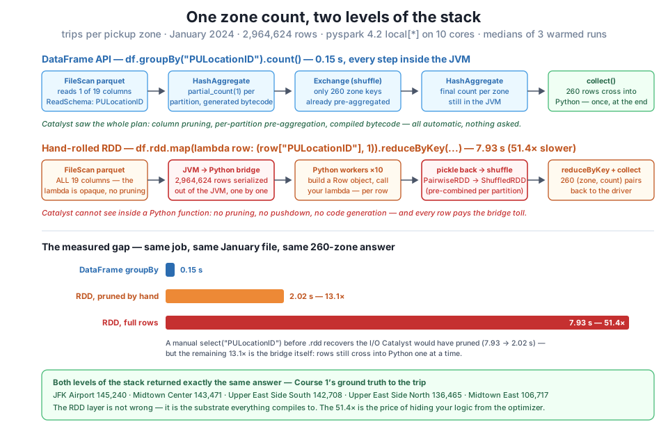
So the 51.4x decomposes cleanly into the two mechanisms the plans exposed. Mechanism one — the blind optimizer: Catalyst optimizes what it can read. A column name in groupBy is legible; a Python lambda is a sealed envelope, so pruning, pushdown, pre-aggregation choices, and code generation all switch off. That cost you could partially claw back by hand (7.93 → 2.02 s), if you remember to, on every query, forever. Mechanism two — the bridge: Python logic can only run in a Python process, so every row must be serialized out of the JVM, materialized as a Row, processed, and its result pickled back. That’s the 13.1x floor, and no hand-tuning touches it — it’s structural. Worth saying plainly: this is not “Python is slow.” It’s per-row boundary-crossing that’s slow. The DataFrame API is also Python — you wrote Python all lesson — but it’s Python that describes work executed in the JVM, rather than Python that performs work row by row.

When RDDs Are Still the Right Tool#

After a 51.4x drubbing, it would be easy to file RDDs under “never.” That’s not the honest verdict. There are three situations where dropping down is still correct engineering.

Data with no schema yet. Raw log lines, scraped text, weird binary records, files so malformed a reader chokes — when structure doesn’t exist until your code creates it, sc.textFile (or binaryFiles) plus map is exactly right. Our zone-lookup parse was this case in miniature: 265 lines, arbitrary Python, no schema until we imposed one. The pattern in the wild is almost always parse at RDD level, then convert to a DataFrame immediately — pay the bridge once to create structure, then live where the optimizer can see.

Fine-grained control over partitioning and placement. The DataFrame API deliberately hides partitions; the RDD API hands you the wheel — custom partitioners, mapPartitions for expensive per-partition setup (open one connection or load one model per partition, not per row), explicit control that a few specialized pipelines genuinely need. If you don’t know you need it, you don’t.

Legacy code. Spark programs written before 2015 — and plenty written after by force of habit — are RDD code, and they still run. Reading them requires exactly the literacy this lesson built; rewriting them against the DataFrame API is usually the single cheapest performance win available, and now you can quote the multiple to justify the ticket.

And when the real need is “custom Python logic on structured data” — the thing people used to reach for RDDs to get — modern Spark has better escape hatches: pandas_udf and friends ship columnar batches across the bridge via Arrow instead of one row at a time, keeping most of the toll unpaid. Module 4 measures exactly what those cost. The modern default stands: logic in the DataFrame API where Catalyst can read it; the RDD layer for the three cases above, and for what Lessons 3 and 4 need it for — a window into what the engine actually executed. Session closed; the meter stops:

spark.stop()

Practice Exercises#

Exercise 1 — The borough scoreboard, both ways. Extend the zone-lookup parse to also build an id -> borough dict (parts[1]). Then count January trips per borough twice: once at RDD level — df.select("PULocationID").rdd, a map that looks each zone up in your dict, reduceByKey — and once at DataFrame level, reading the lookup with spark.read.csv(..., header=True, inferSchema=True) and using a join plus groupBy. Verify the two agree, then compare times under the lesson’s bench policy. Before running, predict: closer to the 13.1x pruned gap or the 51.4x full-row gap, and why?

Exercise 2 — One number, two tolls. Compute January’s total revenue (sum of total_amount, whole raw file, no time filter) twice: df.select("total_amount").rdd.map(lambda r: r[0]).reduce(lambda a, b: a + b) versus df.agg(F.sum("total_amount")) (with from pyspark.sql import functions as F). Time both with the bench policy. Note this is a reduce to a single value, not a reduceByKey — no grouping, minimal shuffle — so before running, predict whether the gap will be larger or smaller than the zone count’s 13.1x pruned gap.

Exercise 3 — Test the folklore fix. A widely-repeated optimization claims mapPartitions beats map because the lambda is called once per partition instead of once per row. Rewrite the full-row zone count with mapPartitions: a function that takes an iterator of rows, tallies zones into a collections.Counter, and yields counter.items(); then reduceByKey and collect as before. Bench it against the plain map version and compute how much of the 7.93 s it recovers.

Summary#

You dropped one level down and put a price on the elevator ride back up. An RDD — resilient, distributed, dataset — is Spark’s original abstraction and its enduring substrate: an immutable, partitioned collection of arbitrary objects with the lineage to recompute any lost piece, sitting under every DataFrame and exposed by df.rdd (January’s showed the same 10 partitions Module 1 measured, holding 2,964,624 Row objects). The API is seductively clean — map, filter, reduceByKey with plain lambdas parsed the 265-zone lookup from raw text in under a second — and the laziness law survives intact at this level: transformations plan, actions pay. Then the measurements. An RDD filter counting JFK pickups matched ground truth exactly (145,240) but took 7.74 s against the DataFrame’s 0.25 s; the full hand-rolled zone count lost 7.93 s to 0.15 s — 51.4x — with all three implementations agreeing digit-for-digit on Course 1’s January podium (JFK 145,240, Midtown Center 143,471, UES South 142,708). The plans explained the gap as two stacked mechanisms: Catalyst reads column names but not lambdas, so the RDD scan pulled all 19 columns where ReadSchema: struct<PULocationID:int> pulled one (hand-pruning recovered that: 7.93 → 2.02 s); and Python logic only runs in Python processes, so every row paid serialization across the JVM→Python bridge — the 13.1x residue no tuning removes. toDebugString showed the receipts: FileScanRDD at the base (DataFrames literally compile to RDDs) and javaToPython feeding an opaque PythonRDD. RDDs remain right for schemaless parsing, partition-level control, and legacy code — and pandas_udf (Module 4) is the modern bridge-toll discount.

Key Concepts#

• RDD (Resilient Distributed Dataset) — Spark’s original core abstraction: an immutable, partitioned collection of arbitrary objects, each partition recomputable from lineage; still the layer every DataFrame plan compiles down to, exposed via df.rdd.
• The JVM→Python bridge — Python lambdas run in separate worker processes (10 here), so RDD code serializes every row out of the JVM and back; that per-row toll was the unremovable 13.1x between a hand-pruned RDD job (2.02 s) and the DataFrame (0.15 s).
• Opaque functions blind the optimizer — Catalyst optimizes what it can read: a groupBy("PULocationID") earned a one-column ReadSchema and JVM-side partial_count; a lambda earned a 19-column scan and zero rewrites, because a Python function is a sealed envelope.
• toDebugString — the RDD-level plan printout: reading it bottom-up revealed FileScanRDD under the DataFrame and the javaToPython → PythonRDD chain that is the bridge; Lesson 4 rereads it as a lineage and fault-tolerance story.
• When RDDs win — schemaless/binary input that needs arbitrary parsing, fine-grained partition control (mapPartitions for per-partition setup), and legacy code — parse low, then climb back up to DataFrames where the optimizer can see.

Why This Matters#

CityFlow will meet this gap in production, not in a textbook — because the 51.4x failure mode is invisible in code review. The hand-rolled zone count is short, readable, idiomatic-looking Python; nothing about it warns that it forces three million rows across a process boundary and switches off the optimizer. Someone on every Spark team eventually writes it (or inherits it from a 2014-era pipeline), and the fix — expressing the same logic in the DataFrame API — is now a change you can argue for with a measured multiple and two plans as evidence, rather than a style preference. The deeper professional skill is the diagnostic reflex this lesson installed: when a Spark job is mysteriously slow, one of your first questions is now “does any step smuggle per-row Python into the plan?” — and you know to look for PythonRDD in the debug string and a fat ReadSchema in the scan. Just as important is the calibrated respect: RDDs aren’t a trap, they’re a layer — the right place to stand when data has no schema yet, and the window Lessons 3 and 4 will look through to watch the engine schedule, shuffle, and remember how to rebuild your work.

Continue Building Your Skills#

You’ve now seen Spark from one level below the API you’ll use daily — and you know what the DataFrame layer is doing for you, in seconds and in plan lines. The next lesson climbs back up and asks the question this one kept deferring: when an action finally fires, what exactly does Spark schedule? Lesson 3, The DAG: Jobs, Stages, Tasks, dissects the execution hierarchy for real — one action becoming jobs, jobs splitting into stages at shuffle boundaries, stages fanning out into one task per partition (you’ve already met the 10) — using the status tracker to catch the engine in the act, and watching Spark 4’s adaptive execution rewrite the plan mid-flight. The Exchange you saw planned at 200 partitions today gets coalesced before your eyes, and the vocabulary of narrow versus wide transformations stops being vocabulary and becomes something you can point to in a running job.