Title here
Summary here
This module has been circling one machine from different sides. Lesson 1 proved Spark is lazy — transformations return in milliseconds because they only build a plan, and the action pays for everything, twice if you call two actions. Lesson 2 went underneath the DataFrame to the RDD and measured what happens when Catalyst can’t see your code. And back in Module 1’s architecture lesson, you met the vocabulary of execution — job, stage, task — and pulled one real aggregation’s anatomy out of the status tracker: two jobs, 21 tasks scheduled, 11 run. What you don’t have yet is the skill that turns that vocabulary from trivia into an engineering tool: given a pipeline you have not yet run, say what Spark will schedule — how many stages, cut where, with how many tasks each — and be right.
That skill has a precise foundation. The plan a lazy DataFrame accumulates is a DAG — a directed acyclic graph of transformations, each node depending on the ones before it — and when an action fires, Spark compiles that graph into physical work using two rules you can apply on paper. Rule one: the job splits into stages wherever data must move between partitions — at the shuffles. Rule two: each stage runs one task per partition of the data it reads. This lesson teaches you to apply those rules before running, then verifies every prediction against Spark’s own bookkeeping — sc.statusTracker(), the same source the Spark UI reads — on CityFlow’s real quarter. Some predictions will hold exactly (10 partitions → 10 tasks, to the task). Some will be wrong in instructive ways, because Spark 4 ships an optimizer that rewrites jobs while they run — and learning to read its output is not optional, because it is what your screen will actually show. By the end, a pipeline’s shape should be something you compute in your head, not something you discover in the logs.
By the end of this lesson, you will be able to:
explain()’s Exchange lines)setJobGroup and read job/stage/task anatomy programmatically from sc.statusTracker()You’ll need pyspark (JDK 17 or 21 — see the course setup) and the three taxi-quarter Parquet files. Paper first, engine second.
Module 1 gave you the four levels; here they are again, but sharpened into rules you can compute with.
An action (count, collect, show, write, toPandas) triggers execution. The textbook says one action makes one job; hold that thought loosely, because Spark 4’s runtime optimizer is allowed to break it, and today you will watch it do so. What never breaks is the direction: jobs come only from actions. A pipeline of pure transformations schedules nothing, ever — that was Lesson 1’s whole measurement.
A job splits into stages, and the cut line is always the same thing: a shuffle — a point where rows must physically move between partitions before work can continue. Everything upstream of the move is one stage; everything downstream is another. Which brings the vocabulary this lesson exists to install, because it is how you find the cut lines by reading code:
A narrow transformation maps each input partition to one output partition, with no data movement. filter reads a partition and emits a smaller one. select and withColumn reshape rows where they sit. drop, cast — same. Chains of narrow transformations fuse into a single stage: Spark runs filter-then-select-then-arithmetic as one pass over each partition, one task per partition, nothing crossing between them.
A wide transformation needs rows regrouped across partitions before it can produce output. groupBy("PULocationID") must gather every zone-132 row (currently scattered across all 10 partitions) into one place before it can count them. join must line up matching keys from two datasets. orderBy must range-slice the whole dataset. distinct and repartition — same. Every wide transformation forces a shuffle, and every shuffle ends a stage.
So the paper procedure is: scan the pipeline, count the wide transformations — that’s the shuffle count — and stages = shuffles + 1. Then size each stage: the first runs one task per input partition; post-shuffle stages default to spark.sql.shuffle.partitions tasks (we’ll print the default in a moment) unless the optimizer resizes them. One honest deferral before we start: this lesson teaches you to find shuffles, not to fear them. What a shuffle costs — the sorting, the disk, the network on a real cluster — is Module 5’s entire subject. Today, a shuffle is a boundary line; in Module 5 it becomes a bill.
The data is CityFlow’s verified quarter — the public NYC TLC Trip Record Data, January through March 2024:
# gate: skip
# CityFlow's verified quarter, fetched once from the public TLC source.
import urllib.request
for month in ("01", "02", "03"):
    urllib.request.urlretrieve(
        f"https://d37ci6vzurychx.cloudfront.net/trip-data/yellow_tripdata_2024-{month}.parquet",
        f"yellow_tripdata_2024-{month}.parquet",
    )
Start the standard session and put the three numbers every prediction in this lesson depends on in front of us:
import warnings
warnings.filterwarnings("ignore")
import time
from pyspark.sql import SparkSession
import pyspark.sql.functions as F

spark = (SparkSession.builder
         .appName("cityflow")
         .master("local[*]")
         .config("spark.ui.showConsoleProgress", "false")
         .getOrCreate())
spark.sparkContext.setLogLevel("ERROR")
sc = spark.sparkContext

jan = spark.read.parquet("yellow_tripdata_2024-01.parquet")
print("defaultParallelism           :", sc.defaultParallelism)
print("January partitions           :", jan.rdd.getNumPartitions())
print("spark.sql.shuffle.partitions :", spark.conf.get("spark.sql.shuffle.partitions"))
defaultParallelism : 10
January partitions : 10
spark.sql.shuffle.partitions : 200Three facts, three roles. defaultParallelism is 10 — local[*] on this 10-core machine, as Module 1 established. January reads as 10 partitions, so any stage that scans January should schedule exactly 10 tasks — that’s rule two, and the tracker is about to grade it. And spark.sql.shuffle.partitions is 200: the configured task count for any stage downstream of a shuffle. Write that one down with suspicion. Two hundred tasks to process a few hundred zone counts would be absurd, and the gap between that configured default and what actually runs is where Spark 4’s runtime optimizer will enter this story.
The Spark UI shows all of this beautifully, but you can’t paste a browser into a script, so we’ll read the same bookkeeping programmatically. Two tools. sc.setJobGroup(id, description) tags every job triggered on the current thread until you clear it — the id is for looking jobs up, and the description is a human label you’ll see in the UI’s Jobs table (there’s also a plain sc.setJobDescription() when you only want the label). sc.statusTracker() answers questions about what ran: which job ids belong to a group, which stages belong to a job, and how many tasks each stage scheduled and completed. Wrap the lookup in a helper we’ll reuse all lesson:
def anatomy(group):
    """Print the job -> stage -> task tree for one tagged group of jobs."""
    tracker = sc.statusTracker()
    scheduled = ran = 0
    for job_id in sorted(tracker.getJobIdsForGroup(group)):
        job = tracker.getJobInfo(job_id)
        print(f"job {job_id}: {len(job.stageIds)} stage(s)")
        for stage_id in sorted(job.stageIds):
            stage = tracker.getStageInfo(stage_id)
            scheduled += stage.numTasks
            ran += stage.numCompletedTasks
            note = "  <- skipped" if stage.numCompletedTasks == 0 else ""
            print(f"  stage {stage_id}: {stage.numTasks} tasks scheduled, "
                  f"{stage.numCompletedTasks} ran{note}")
    print(f"group total: {scheduled} tasks scheduled, {ran} ran")
The helper prints the hierarchy exactly as this lesson defined it — jobs containing stages, stages containing task counts — plus one distinction that will matter immediately: tasks scheduled versus tasks that actually ran. In a healthy textbook world those are equal. Keep an eye on them.
First prediction. Take a pipeline of purely narrow transformations — a filter (rows stay in their partitions, fewer of them) and a select (columns drop, rows don’t move) — and end it with count(). On paper: narrow transformations fuse into one stage, January is 10 partitions, so the naive call is one job, one stage, 10 tasks. Run it and grade yourself:
sc.setJobGroup("narrow", "JFK trips: filter + select + count")
t0 = time.perf_counter()
jfk = (jan.filter(F.col("PULocationID") == 132)
          .select("PULocationID", "total_amount")
          .count())
sc.setJobGroup(None, None)
print(f"JFK January pickups: {jfk:,}  ({time.perf_counter() - t0:.2f} s)")
anatomy("narrow")
JFK January pickups: 145,240 (3.48 s)
job 1: 1 stage(s)
stage 1: 10 tasks scheduled, 10 ran
job 2: 2 stage(s)
stage 2: 10 tasks scheduled, 0 ran <- skipped
stage 3: 1 tasks scheduled, 1 ran
group total: 21 tasks scheduled, 11 ranThe answer is right — 145,240 JFK pickups, exactly Course 1’s verified January figure (the 3.48 s includes a fresh session’s first-job warm-up; Module 1 measured that fixed cost). The prediction is wrong twice: two jobs, and three stages where we predicted one. Recognize the totals, though — 21 scheduled, 11 ran is precisely the anatomy Module 1’s lesson measured for a groupBy-and-collect. Our supposedly boundary-free pipeline produced the same shape as an aggregation. Two suspects to interrogate.
Suspect one: the action itself. count() is not a free readout — it is an aggregation. Each of the 10 tasks counts its own partition’s surviving rows, and those 10 partial counts must then be brought together into one number. Bringing partial results together is a regrouping — a shuffle boundary, structurally identical to a groupBy’s, even though only 10 integers cross it. The 10-task stage is our fused narrow pipeline computing partial counts; the 1-task stage is the merge. The narrow transformations added no boundary, exactly as promised. The action’s answer-assembly added one. Refine the paper rule accordingly: stages = shuffles + 1, counting the action’s own final merge as a shuffle when it aggregates — count does, collect doesn’t (it just ships each partition’s rows to the driver).
Suspect two: the optimizer that re-plans mid-flight. That explains three stages, but not two jobs, and not a stage that scheduled 10 tasks and ran zero. This is adaptive query execution (AQE), on by default in Spark 4, and here is the honest one-paragraph version: instead of executing the whole plan blind, Spark runs it piecewise — it executes up to a shuffle boundary, materializes the shuffle output, looks at the runtime statistics (real sizes, real row counts, not estimates), re-plans everything downstream with that knowledge, and submits the remainder as a new job. The new job’s plan still contains the upstream stages, so they appear in its bookkeeping — scheduled — but their output already exists, so Spark skips them: 10 tasks scheduled, 0 ran. That’s job 2’s stage 2. And AQE’s best-known rewrite is exactly the one your suspicious note predicted: the post-shuffle stage that spark.sql.shuffle.partitions configured at 200 tasks got coalesced to 1, because runtime statistics said 10 partial counts don’t need 200 workers. So: 21 scheduled, 11 ran, one honest number returned. AQE is not noise to explain away — it is Spark choosing a better plan than the config file’s guess, and every job you run in this course will wear its fingerprints.
Why the job numbers skip
Our first tagged job is job 1, not job 0 — and later groups will skip numbers too. Nothing is lost: job ids are application-wide and count every job, including small untagged housekeeping ones (opening Parquet inputs and probing partition layouts run tiny jobs of their own). The tracker’s group lookup is exactly how you stay oriented: tag what you care about, query the tag, ignore the rest.
Good experimental method: we claimed the boundary came from count()’s merge, not from our transformations. Remove the merge and check. Spark ships a noop write format — a data sink that runs the full pipeline and throws the output away, no files, no result to assemble. It exists for exactly this kind of benchmarking. If the narrow-pipeline theory is right, the same filter-and-select into a no-op sink should be the pure shape: one job, one stage, 10 tasks, nothing skipped, nothing merged.
sc.setJobGroup("pipeline-only", "same narrow pipeline, no-op sink")
(jan.filter(F.col("PULocationID") == 132)
    .select("PULocationID", "total_amount")
    .write.format("noop").mode("overwrite").save())
sc.setJobGroup(None, None)
anatomy("pipeline-only")
job 3: 1 stage(s)
stage 4: 10 tasks scheduled, 10 ran
group total: 10 tasks scheduled, 10 ranTheory confirmed, cleanly. One job, one stage, 10 tasks — one per partition — all run, none skipped. No shuffle anywhere, so AQE had no boundary to pause at and nothing to re-plan; the “2 jobs” behavior vanished along with the merge. This is the platonic narrow pipeline the paper rule describes, and it earns you a sharper mental model: the transformations decide the boundaries inside the data flow; the action decides whether one more regrouping is appended at the end. Filter and select move nothing. Count merges. collect ships. write (a real one) streams each partition to its own output file — still no regrouping. Keep the noop sink in your kit: it is the cheapest way to ask “what does my pipeline cost, apart from delivering the answer?”
Now put a genuinely wide transformation in the middle and watch the boundary move from the action into the data flow. groupBy("PULocationID").count() must regroup rows by zone — that’s a shuffle by the transformation’s nature, and it would be there no matter which action followed. Prediction, AQE-aware this time: a 10-task scan stage computing per-partition partial counts, a boundary, then a merge stage that AQE will coalesce down from 200 — and because AQE pauses at the boundary, expect it packaged as two jobs with a skipped stage:
sc.setJobGroup("wide", "zone counts, January")
zones = jan.groupBy("PULocationID").count().collect()
sc.setJobGroup(None, None)
top3 = sorted(zones, key=lambda r: -r["count"])[:3]
print(f"{len(zones)} zones came back")
for r in top3:
    print(f"  zone {r['PULocationID']}: {r['count']:,} trips")
anatomy("wide")
260 zones came back
zone 132: 145,240 trips
zone 161: 143,471 trips
zone 237: 142,708 trips
job 4: 1 stage(s)
stage 5: 10 tasks scheduled, 10 ran
job 5: 2 stage(s)
stage 6: 10 tasks scheduled, 0 ran <- skipped
stage 7: 1 tasks scheduled, 1 ran
group total: 21 tasks scheduled, 11 ranPrediction: perfect this time. Ten-task scan (job 4), boundary, skipped repeat, one-task coalesced finish (job 5) — 21 scheduled, 11 ran. And the answers are Course 1’s verified January podium to the trip: JFK (132) 145,240, Midtown Center (161) 143,471, Upper East Side South (237) 142,708, across 260 distinct pickup zones.
Sit with an uncomfortable observation for a moment: this anatomy is identical to the narrow-count’s. Same stage counts, same task totals. If shapes match, why does the narrow/wide vocabulary matter? Because of what the boundary is made of and what crosses it. The count’s boundary moved 10 integers; this one moves each task’s partial table of up-to-260 zone counts — still kilobytes, which is why AQE coalesced both to a single finisher, but the volume crossing a groupBy’s boundary scales with the data and the key count, while a count’s merge never grows past one number per task. On this quarter, at these sizes, the difference is invisible. In Module 5, with wider keys and real volumes, the difference is the whole performance story — which is exactly why the skill being drilled here is finding the boundaries, not yet pricing them. A join and an orderBy cut stages the same way; you’ll predict one of each before this module ends.
Everything anatomy() prints, the Spark UI draws — and while the session is alive, it’s one browser tab away at http://localhost:4040 (check sc.uiWebUrl if another session grabbed the port first). Two pages matter for this lesson.
The Jobs page is the tracker made visual: every job, its stages, and — because we set them — our setJobGroup descriptions in the Description column, which is what makes a busy application’s job list navigable. Click any job and you get its DAG Visualization: the job’s stages drawn as boxes, the operators inside each box (Scan parquet, Filter, Project, HashAggregate, Exchange…), and arrows crossing between boxes exactly where the shuffles are. Skipped stages render grey — the UI’s honest way of drawing “scheduled but reused.” Pull up job 5 and you are looking at this lesson’s whole argument as a picture: a grey 10-task box feeding a colored 1-task box across a shuffle boundary.
The SQL / DataFrame page shows the query-level view — one entry per action, with the full operator DAG and, after the run, AdaptiveSparkPlan isFinalPlan=true: the plan as AQE actually finalized it, including an AQEShuffleRead node where 200 partitions became 1. Module 4 teaches you to read plan text in anger; for now, know that the picture of “what did AQE change?” lives on this page.
The tracker and the UI die with the session
Both sc.statusTracker() and port 4040 are served by your live driver — spark.stop() takes the bookkeeping with it, so query and browse during the run (a input("Enter to finish") before stop() buys you time). Real clusters run a history server that persists this UI after applications end; your laptop just forgets. One more honesty note: the tracker retains a bounded window of recent stages, so query anatomy right after the job, not hundreds of jobs later.
Time to earn the lesson’s skill statement on a pipeline with real structure: CityFlow’s quarter zone leaderboard. Filter the quarter to Course 1’s report window (Course 1 established that 21 stray-stamped trips fall outside it), count trips per pickup zone, and rank zones busiest-first. Read the code as a stage-counter would, before running anything:
QUARTER = ["yellow_tripdata_2024-01.parquet",
           "yellow_tripdata_2024-02.parquet",
           "yellow_tripdata_2024-03.parquet"]
quarter = spark.read.parquet(*QUARTER)
print("quarter partitions:", quarter.rdd.getNumPartitions())

leaderboard = (quarter
    .filter((F.col("tpep_pickup_datetime") >= "2024-01-01") &
            (F.col("tpep_pickup_datetime") < "2024-04-01"))
    .groupBy("PULocationID").count()
    .orderBy(F.desc("count")))
leaderboard.explain()
quarter partitions: 10
== Physical Plan ==
AdaptiveSparkPlan isFinalPlan=false
+- Sort [count#69L DESC NULLS LAST], true, 0
+- Exchange rangepartitioning(count#69L DESC NULLS LAST, 200), ENSURE_REQUIREMENTS, [plan_id=150]
+- HashAggregate(keys=[PULocationID#56], functions=[count(1)])
+- Exchange hashpartitioning(PULocationID#56, 200), ENSURE_REQUIREMENTS, [plan_id=147]
+- HashAggregate(keys=[PULocationID#56], functions=[partial_count(1)])
+- Project [PULocationID#56]
+- Filter ((isnotnull(tpep_pickup_datetime#50) AND (tpep_pickup_datetime#50 >= 2024-01-01 00:00:00)) AND (tpep_pickup_datetime#50 < 2024-04-01 00:00:00))
+- FileScan parquet [tpep_pickup_datetime#50,PULocationID#56] ...(The FileScan line’s path and pushed-filter details are trimmed for width.) On paper: filter is narrow — no boundary, it fuses into the scan. groupBy is wide — boundary one. orderBy is wide — boundary two. Two shuffles, so three stages: a 10-task scan (the quarter read as 10 partitions), an aggregation stage, a sort stage — the last two configured at 200 tasks each. And explain() agrees, in its own dialect: read it bottom-up and there are exactly two Exchange operators — Spark’s plan-language for shuffle — one hashpartitioning by zone (the groupBy) and one rangepartitioning by count (the sort). Counting Exchanges in a plan and counting wide transformations in code are the same act. Note also AdaptiveSparkPlan isFinalPlan=false: the plan itself is telling you it’s a draft that AQE will finish at runtime. So the AQE-aware prediction: same three stages’ worth of work, cut into more jobs at the two boundaries, repeats skipped, the 200s coalesced to something honest. Run it:
sc.setJobGroup("exam", "quarter zone leaderboard")
t0 = time.perf_counter()
rows = leaderboard.collect()
sc.setJobGroup(None, None)
print(f"{len(rows)} zones, {sum(r['count'] for r in rows):,} trips kept  "
      f"({time.perf_counter() - t0:.2f} s)")
for r in rows[:3]:
    print(f"  zone {r['PULocationID']}: {r['count']:,} trips")
anatomy("exam")
262 zones, 9,554,757 trips kept (2.79 s)
zone 161: 453,825 trips
zone 237: 439,138 trips
zone 132: 429,745 trips
job 7: 1 stage(s)
stage 9: 10 tasks scheduled, 10 ran
job 8: 2 stage(s)
stage 10: 10 tasks scheduled, 0 ran <- skipped
stage 11: 1 tasks scheduled, 1 ran
job 9: 2 stage(s)
stage 12: 10 tasks scheduled, 0 ran <- skipped
stage 13: 1 tasks scheduled, 1 ran
job 10: 3 stage(s)
stage 14: 10 tasks scheduled, 0 ran <- skipped
stage 15: 1 tasks scheduled, 0 ran <- skipped
stage 16: 1 tasks scheduled, 1 ran
group total: 44 tasks scheduled, 13 ranTruth first: 9,554,757 trips kept — Course 1’s report window figure exactly (21 quarantined from 9,554,778) — and the podium is Course 1’s verified quarter answer to the trip: Midtown Center (161) 453,825, Upper East Side South (237) 439,138, JFK (132) 429,745, across 262 zones. Same data, same window, new engine, same truth.
Now grade the prediction. The three stages of real work are all here: the 10-task scan-filter-partial-count (stage 9, job 7), the aggregation finish coalesced 200→1 (stage 11, job 8), the sort coalesced 200→1 (stage 16, job 10). Boundaries: exactly where the two Exchanges said, and nowhere else — the filter added none. Task rule: 10 partitions, 10 scan tasks, to the task. But the packaging holds one last surprise: four jobs, not three. Job 9 — a skipped scan plus one real task — is the sort’s preparation pass. A range sort has to decide where to slice the data into sorted ranges, and to do that Spark first samples the sort keys (that’s what rangepartitioning needs to stay balanced); with the aggregated counts already materialized at one partition, that sampling was a single cheap task. It’s a good final exhibit for the lesson’s honest theme: the boundaries were 100% predictable from the code; the packaging — how many jobs, what gets skipped, how post-shuffle stages are sized, whether a sampling pass appears — belongs to the runtime. Predict the first; read the second. Total: 44 tasks scheduled, 13 actually run, and every one of the 31 skipped was work AQE proved it didn’t need to redo.
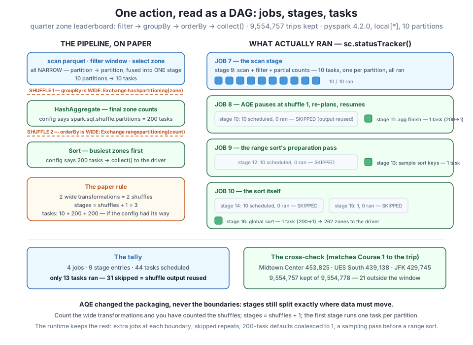
collect(), read as a DAG — quarter zone leaderboard (filter → groupBy → orderBy) over 9,554,757 kept trips, pyspark 4.2.0, local[*]. On paper (left): the narrow filter/select fuse into the scan; two wide transformations mean two shuffles (Exchange hashpartitioning, Exchange rangepartitioning in the plan) and therefore three stages — 10 scan tasks (one per partition) plus two stages the config sizes at 200 tasks each. As run (right): adaptive query execution kept every boundary but re-cut the packaging into 4 jobs — the 10-task scan, a skipped repeat plus a 1-task aggregation finish (AQE coalesced 200→1), a 1-task sampling pass to balance the sort ranges, and a 1-task final sort — 44 tasks scheduled, 13 ran, with all 31 skipped tasks being shuffle output AQE reused. The podium matches Course 1's ground truth to the trip: Midtown Center 453,825 · UES South 439,138 · JFK 429,745.The measuring is done — close the application:
spark.stop()
print("session closed -- the DAG pages at localhost:4040 went down with it")
session closed -- the DAG pages at localhost:4040 went down with itAnd here is your new superpower, stated as the procedure you’ll rehearse in this module’s guided project. Given any DataFrame pipeline: (1) classify each transformation — narrow ones fuse, wide ones cut; (2) stages = shuffles + 1, adding one more if the action itself merges (a count, an agg without keys); (3) first stage runs one task per input partition — a number you can check with df.rdd.getNumPartitions() before running anything; (4) post-shuffle stages are configured at spark.sql.shuffle.partitions but expect AQE to right-size them from runtime statistics, splitting the work into extra jobs with skipped stages along the way, plus a sampling pass if anything range-sorts. Say it before you run it; let the tracker grade you.
Exercise 1 — Classify, predict, verify. For each of these three January pipelines, write down the full prediction first — narrow or wide for each transformation, number of shuffles, number of stages, tasks in the first stage, and whether you expect AQE to split jobs — then run each under its own setJobGroup tag and grade yourself with anatomy(): (a) jan.withColumn("tip_pct", F.col("tip_amount") / F.col("total_amount")).filter(F.col("tip_pct") > 0.3).select("PULocationID", "tip_pct") written to the noop sink; (b) jan.select("payment_type").distinct().collect(); (c) jan.repartition(4).count().
Hint
Work the vocabulary: withColumn, filter, select are all narrow — (a) should reproduce the lesson’s purest shape. distinct is secretly a groupBy on every selected column, so (b) is wide and should wear the familiar two-job, skipped-stage, coalesced-finish anatomy. repartition(4) is wide by definition — its entire job is moving rows — so (c) has a shuffle before the count’s own merge even starts; predict the middle stage’s task count from the argument you passed, not from the 200 default, and check whether AQE respects an explicit repartition (it does — you asked for 4 on purpose).
Exercise 2 — Turn AQE off and meet the textbook. Set spark.conf.set("spark.sql.adaptive.enabled", "false"), rebuild the quarter leaderboard pipeline from spark.read.parquet onward, and collect it under a fresh job group. Compare the anatomy against the lesson’s: how many jobs now, how many stages, and — the headline — how many tasks did the two post-shuffle stages run this time? Compute the ratio of tasks run (AQE off vs on), then decide which plan you’d rather operate. Set the flag back to "true" when done.
Hint
Rebuild the DataFrame after flipping the flag — the setting is read when a query plans, so reusing the old leaderboard object risks measuring a stale plan. Expect the textbook picture this lesson’s paper rules describe: the boundaries in the same two places, but the aggregation and sort stages running at the configured 200 tasks each — hundreds of tasks to shepherd 262 rows — plus the range-sort’s sampling job, which exists with or without AQE. The run may not even be slower at this scale (tasks are cheap when partitions are tiny); the point is the waste you can now see and count. Turning AQE off temporarily is a legitimate learning tool and a bad production habit.
Exercise 3 — Read the DAG where it’s drawn. Wrap the leaderboard collect() in a loop of 20 runs so the application stays alive, open http://localhost:4040, and bring back four written observations: (1) your job-group description in the Jobs table, and which job ids it spans; (2) the final job’s DAG Visualization — how many stage boxes, which are grey, and which operator names appear inside the box that actually ran; (3) on the 10-task scan stage’s detail page, the Shuffle Write column’s total size — write the number down and reflect on how small it is for 9.5 million input rows; (4) on the SQL / DataFrame page, the query’s plan with isFinalPlan=true — find the AQEShuffleRead node and note what it says about partition counts.
Hint
Keep the script running or the UI vanishes — either browse mid-loop or park input("Enter to stop") before spark.stop(). Grey boxes are skipped stages: the UI drawing the tracker’s 0 ran. For (3), the shuffle write is tiny because the scan stage already did partial aggregation — each task emits at most one row per zone it saw, not its millions of input rows; that “combine before you move” trick is a load-bearing optimization Module 5 dissects. For (4), isFinalPlan=true appears only after the action completes — AQE finalizes plans by running them, which is the whole idea of this lesson in one flag.
An action triggers execution, and what executes is a DAG compiled into a hierarchy you can now predict: jobs, cut into stages wherever data must move, each stage running one task per partition. The cut lines are readable straight from code — narrow transformations (filter, select, withColumn) map partition to partition and fuse into a single stage, while wide ones (groupBy, join, orderBy, distinct, repartition) force a shuffle — or from a plan, where every Exchange in explain() is a boundary. The tracker graded the paper rules honestly: a narrow filter-and-select into a noop sink ran the pure shape (1 job, 1 stage, 10 tasks over January’s 10 partitions), but ending the same pipeline with count() produced 2 jobs and 21 scheduled tasks — the action’s own answer-merge is a boundary, and adaptive query execution re-plans at every boundary using runtime statistics, splitting jobs, skipping already-materialized stages (10 scheduled, 0 ran), and coalescing the configured 200 post-shuffle tasks to 1. A wide groupBy wore the identical 21-scheduled/11-ran anatomy while returning Course 1’s exact January podium (JFK 145,240). The final exam — filter + groupBy + orderBy over the quarter window — proved the split of labor: both boundaries sat exactly where the two Exchanges predicted, the scan ran exactly 10 tasks, and the packaging belonged to the runtime: 4 jobs (one a range-sort sampling pass), 44 tasks scheduled, 13 run, and a leaderboard matching ground truth to the trip — 9,554,757 kept, Midtown Center 453,825, UES South 439,138, JFK 429,745. Predict the boundaries; read the packaging.
filter, select, withColumn) and fuses; wide must regroup rows across partitions (groupBy, join, orderBy, distinct, repartition) and always cuts a stage. The vocabulary that turns code review into stage counting.setJobGroup + sc.statusTracker() — the instrumentation pair: tag the work, then read jobs, stages, and scheduled-vs-ran task counts programmatically — the same bookkeeping the UI’s DAG Visualization draws, alive only while the session is.CityFlow’s engineers review each other’s pipelines in exactly the terms this lesson drilled. “This backfill has three shuffles and the middle one regroups the full fact table” is a code-review comment that saves cluster-hours; being able to make it requires nothing more than the classification you just practiced — and being unable to make it means discovering the third shuffle in production, at 2 a.m., from a stage that won’t finish. The prediction habit also keeps you honest with the optimizer: engineers who can’t predict a job’s shape treat AQE’s extra jobs and skipped stages as mysteries or, worse, as bugs to disable; engineers who can predict the boundaries recognize the packaging for what it is — the runtime spending statistics you didn’t have at plan time. And the payoff compounds next module and beyond: Module 5’s shuffle-cost work assumes you can already find every shuffle in a pipeline at a glance, because you can’t minimize what you can’t locate. This module’s guided project makes the rehearsal formal — prediction sheet first, tracker second.
One thread from today deliberately dangled: those skipped stages worked because Spark knew it could reuse stage output — it kept the recipe and the receipts. That bookkeeping has a name, and it is the subject of Lesson 4, Immutability & Lineage. Every transformation you’ve written returns a new DataFrame rather than modifying the old one, and that’s not a stylistic quirk — immutability is what makes the DAG trustworthy: because no node’s data can change underneath it, Spark can recompute any partition of any DataFrame from source by replaying its lineage — which is the entire fault-tolerance story (recompute, don’t replicate) and the reason a lost executor on a real cluster costs a re-run of a few tasks, not a restarted job. You’ll print real lineage with toDebugString, contrast Spark’s no-aliasing world with pandas’ in-place habits, and revisit Lesson 1’s twice-run trap with sharper eyes: a long lineage replayed per action is a cost you’ll soon want to manage. Bring today’s vocabulary — lineage is just the DAG, remembered.
Keep DATATWEETS free. Help fund practical data, AI, and engineering lessons for learners worldwide.
