Title here
Summary here
Module 2 has been circling one design decision from three directions. Lesson 1 showed you when Spark works — transformations build plans, actions execute them, and two actions on one frame run the whole pipeline twice. Lesson 2 showed you what it works on — RDDs, the partitioned collections underneath every DataFrame. Lesson 3 showed you how the work is organized — jobs split into stages at shuffles, stages split into one task per partition. This lesson answers the question all three left hanging: why is every one of those structures read-only? You have already noticed the symptom. Nothing in three lessons of Spark code ever modified anything: no inplace=True, no assigning into a column, no del df["col"]. Every operation handed back a new DataFrame and left the old one standing. For a pandas user that feels like a missing feature. It is the opposite — it is the feature.
This lesson demonstrates the claim instead of asserting it, on CityFlow’s real quarter. First, immutability itself: filter January’s 2,964,624 trips down to 145,240 airport pickups, recount the original, and find it untouched — then watch pandas 3.0 throw a ChainedAssignmentError at the exact habit Spark makes structurally impossible. Second, what immutability costs: there is no “change one value,” only “build a new frame with the value changed,” and you will do it properly with withColumn and when on the quarter’s famously dirty trip_distance column. Third, what Spark buys with the constraint: lineage. An immutable frame plus the recorded chain of transformations that produced it is a recipe — enough information to recompute any partition from the source files, which is how Spark survives losing work without keeping copies of anything. You will print a real lineage tree with toDebugString, watch explain() grow as transformations stack, and measure recomputation happening on this machine: the same recipe replayed per action, exactly as Lesson 1’s twice-run trap predicted — plus one honest surprise where Spark quietly reuses finished work you never asked it to keep.
By the end of this lesson, you will be able to:
SettingWithCopyWarning, chained assignment) cannot exist in SparkwithColumn + when/otherwise, without touching the source framedf.rdd.toDebugString() — indentation as stage boundaries, (10) and (1) as partition counts — and match it to the explain() planYou’ll need pyspark and pandas — pandas only to show what Spark is not. One session for the whole lesson.
The standard CityFlow block — by now this is muscle memory:
import warnings
warnings.filterwarnings("ignore")
import time

from pyspark.sql import SparkSession
from pyspark.sql import functions as F

spark = (SparkSession.builder
         .appName("cityflow")
         .master("local[*]")
         .config("spark.ui.showConsoleProgress", "false")
         .getOrCreate())
spark.sparkContext.setLogLevel("ERROR")
print("Spark", spark.version, "ready")
Spark 4.2.0 readyKeep the Spark UI tab (http://localhost:4040) open if you like — the recomputation experiments later in this lesson each appear as separate jobs there, which is its own kind of proof.
Start with the strongest version of the claim: you cannot modify a Spark DataFrame. Not “shouldn’t” — cannot. There is no API for it. Every operation that looks like a modification is a transformation, and every transformation returns a new frame. Prove it on January:
jan = spark.read.parquet("yellow_tripdata_2024-01.parquet")
print(f"jan rows              : {jan.count():,}")

airport = jan.filter(F.col("PULocationID") == 132)
print(f"airport rows          : {airport.count():,}")
print(f"jan rows, after filter: {jan.count():,}")
print(f"airport is jan        : {airport is jan}")
jan rows : 2,964,624
airport rows : 145,240
jan rows, after filter: 2,964,624
airport is jan : FalseThree familiar numbers and one telling boolean. January is 2,964,624 rows — Course 1’s verified count. The filter produced 145,240 JFK pickups — exactly the January figure both engines have agreed on since Lesson 3 of Module 1. And jan, recounted after the filter, is still 2,964,624: the filter did not remove rows from jan, it described a new frame that omits them. airport is jan returns False because they are genuinely different Python objects — filter constructed and returned a second DataFrame rather than editing the first.
The same holds for operations that sound like edits. withColumn reads as “add a column to this frame.” It does no such thing:
tagged = jan.withColumn("is_airport", F.col("PULocationID") == 132)
print(f"tagged columns : {len(tagged.columns)}")
print(f"jan columns    : {len(jan.columns)}")
tagged columns : 20
jan columns : 19tagged has 20 columns; jan still has its original 19. Nineteen columns went in, and nineteen are still there — withColumn returned a new frame with the extra column. If you have ever written df.withColumn("x", ...) on its own line and wondered why df had no column x afterward, this is why: the result went nowhere. In Spark you always capture the return value — df = df.withColumn(...) — and as you’ll see shortly, that reassignment costs almost nothing, because frames are plans, not copies.
If you came from pandas, immutability is the un-learning half of this lesson. pandas was built on the opposite instinct: DataFrames are mutable buffers, and mutation is everywhere — inplace=True, df["col"] = ..., del df["col"], assigning into slices. Mutation plus aliasing — two names that may or may not point at the same underlying data — produced one of the most notorious bug classes in data work: chained assignment, the thing SettingWithCopyWarning spent a decade warning about. Write df[mask]["col"] = value and, in classic pandas, the answer to “did that update df?” was it depends — on whether the slice was a view or a copy, which depended on memory layout you couldn’t see. Sometimes it updated. Sometimes it silently didn’t. Pipelines shipped with both behaviors in them.
Here is where that story stands today, on the pandas 3.0.3 installed in this very environment. We silenced warnings at the top of the lesson, so re-enable them locally and try the classic mistake:
import pandas as pd

pdf = pd.DataFrame({"zone": [132, 161, 237],
                    "trips": [145240, 143471, 142708]})

with warnings.catch_warnings(record=True) as caught:
    warnings.simplefilter("always")
    pdf[pdf["zone"] == 132]["trips"] = 0   # the classic chained assignment
    for c in caught:
        print(f"{c.category.__name__}: {str(c.message).splitlines()[0]}")

print(pdf.to_string(index=False))
ChainedAssignmentError: A value is being set on a copy of a DataFrame or Series through chained assignment.
zone trips
132 145240
161 143471
237 142708Zone 132 still shows 145,240 — the write went nowhere, and pandas said so. That warning name is worth a pause: not SettingWithCopyWarning but ChainedAssignmentError, because pandas 3.0 adopted copy-on-write as its only mode, and under copy-on-write, chained assignment never works — deterministically, rather than depending on invisible memory layout. In other words: after twenty years of view-versus-copy bugs, pandas itself concluded that letting two names share mutable data was the mistake, and moved toward exactly the discipline Spark started with.
Spark’s version of the discipline is absolute, and now you can see why the demonstration above was airtight. jan.filter(...) cannot alias jan’s data in any way that matters, because nothing can write to either frame — there is no write. The entire question “view or copy?” is unaskable. That is what “immutability prevents a bug class structurally” means: not that Spark catches the bug, but that the bug has no grammar to be written in.
What pandas’ copy-on-write actually concedes
pandas 3.0’s copy-on-write is a half-step to where Spark lives. Under CoW, every pandas operation behaves as if it returned an independent copy (sharing memory secretly until a write forces a real copy) — which is why the chained write above becomes a guaranteed no-op instead of a maybe. But pandas frames are still mutable through the front door: pdf.loc[pdf["zone"] == 132, "trips"] = 0 works fine and updates in place. Spark closes that door too. If your team is on pandas 2.x, the same code may raise the old SettingWithCopyWarning and — worse — may sometimes actually mutate; that nondeterminism is precisely the historical mess both engines have now, in their different ways, engineered out.
Constraints are only interesting if you also price them. Immutability’s price is this: there is no such thing as updating a value in place. “Fix these cells” must be expressed as “build a new frame in which these cells are different.” Course 1 flagged the quarter’s trip_distance as the dirtiest column in the dataset, so use it for a real repair. First, the damage, on the full quarter:
quarter = spark.read.parquet("yellow_tripdata_2024-01.parquet",
                             "yellow_tripdata_2024-02.parquet",
                             "yellow_tripdata_2024-03.parquet")

print(f"claims over 100 mi : {quarter.filter(F.col('trip_distance') > 100).count()}")
print(f"max trip_distance  : {quarter.agg(F.max('trip_distance')).first()[0]:,}")
claims over 100 mi : 252
max trip_distance : 312,722.3There it is — Course 1’s ground-truth absurdity, reproduced by the second engine: a yellow cab claiming 312,722.3 miles, with 252 trips over 100 miles in total. The immutable repair is withColumn plus when/otherwise: when the distance is implausible, null it out; otherwise keep it. Giving the new column the same name as an old one is how “replace a column” is spelled:
capped = quarter.withColumn(
    "trip_distance",
    F.when(F.col("trip_distance") > 100, None)
     .otherwise(F.col("trip_distance")))

print(f"capped   : max {capped.agg(F.max('trip_distance')).first()[0]}, "
      f"nulls {capped.filter(F.col('trip_distance').isNull()).count()}")
print(f"original : max {quarter.agg(F.max('trip_distance')).first()[0]:,}, "
      f"nulls {quarter.filter(F.col('trip_distance').isNull()).count()}")
capped : max 99.77, nulls 252
original : max 312,722.3, nulls 0capped tops out at a plausible 99.77 miles with exactly 252 nulls — one per repaired cell. And quarter is pristine: max still 312,722.3, zero nulls. Both frames exist simultaneously; neither threatens the other. This is the pattern for every “edit” you will ever make in Spark — fix a category label, cap an outlier, backfill a null: when picks the rows, otherwise passes the rest through, withColumn builds the new frame, and the source stays exactly as the source was. (Notice what it is not: a copy. capped is a plan — no second 160 MB materialized anywhere. That is the next section’s subject.)
Now the payoff side of the ledger. Ask what Spark actually has after a chain of transformations. Not data — the actions above computed results and threw the row streams away. What each frame holds is: a pointer to its parent frame, and the transformation that derives it from that parent. Follow the pointers back and every frame bottoms out at source files on disk. That chain is called lineage, and it means any frame — and any partition of any frame — can be recomputed from scratch, mechanically, by replaying its recipe. Immutability is what makes the recipe trustworthy: since no step can be modified after the fact, a recipe written once is valid forever.
Build a real one — CityFlow’s zone-revenue report for the quarter, five frames deep, and time the build:
t0 = time.perf_counter()
in_window = quarter.filter(
    (F.col("tpep_pickup_datetime") >= "2024-01-01") &
    (F.col("tpep_pickup_datetime") < "2024-04-01"))
flagged = in_window.withColumn("is_reversal", F.col("total_amount") < 0)
by_zone = flagged.groupBy("PULocationID").agg(
    F.count("*").alias("trips"),
    F.sum("total_amount").alias("revenue"),
    F.sum(F.col("is_reversal").cast("int")).alias("reversals"))
report = by_zone.orderBy(F.col("trips").desc())
build_ms = (time.perf_counter() - t0) * 1000
print(f"four frames built and reassigned in {build_ms:.0f} ms -- plans, not copies")
four frames built and reassigned in 309 ms -- plans, not copiesFour new DataFrames over 9.5 million rows in 309 ms, and not one row moved — each variable is a named step in a recipe, not a container of data. This is why the idiomatic Spark style of reassigning freely (df = df.filter(...) then df = df.withColumn(...)) is safe and cheap: safe because the old frame can’t be corrupted by the new one, cheap because “creating a DataFrame” means appending a step to a plan. Naming intermediate steps, as we did here, costs nothing extra and buys you inspectable checkpoints — like these.
Watch the recipe grow with explain(). The source frame’s plan is one step (output trimmed here and below: long column lists and file paths shortened to ...):
quarter.explain()== Physical Plan ==
*(1) ColumnarToRow
+- FileScan parquet [VendorID#90,tpep_pickup_datetime#91,...,Airport_fee#108] Batched: true,
DataFilters: [], Format: Parquet, Location: InMemoryFileIndex(3 paths)[...],
PartitionFilters: [], PushedFilters: [], ReadSchema: struct<...>One step: scan three Parquet files. Add the window filter and the plan gains a layer:
in_window.explain()== Physical Plan ==
*(1) Filter ((isnotnull(tpep_pickup_datetime#91) AND (tpep_pickup_datetime#91 >= 2024-01-01 00:00:00))
AND (tpep_pickup_datetime#91 < 2024-04-01 00:00:00))
+- *(1) ColumnarToRow
+- FileScan parquet [VendorID#90,...,Airport_fee#108] Batched: true,
DataFilters: [isnotnull(tpep_pickup_datetime#91), (tpep_pickup_datetime#91 >= 2024-01-01 00:00:00), ...],
Format: Parquet, Location: InMemoryFileIndex(3 paths)[...],
PushedFilters: [IsNotNull(tpep_pickup_datetime), GreaterThanOrEqual(tpep_pickup_datetime,2024-01-01T00:00), Less...],
ReadSchema: struct<...>The Filter sits on top of the scan — and notice PushedFilters is no longer empty: Catalyst, which Lesson 2 showed can see through DataFrame expressions (and cannot see through Python lambdas), has already pushed the window condition down into the Parquet reader. The full five-step recipe:
report.explain()== Physical Plan ==
AdaptiveSparkPlan isFinalPlan=false
+- Sort [trips#256L DESC NULLS LAST], true, 0
+- Exchange rangepartitioning(trips#256L DESC NULLS LAST, 200), ENSURE_REQUIREMENTS, [plan_id=444]
+- HashAggregate(keys=[PULocationID#97], functions=[count(1), sum(total_amount#106), sum(cast(is_reversal#255 as int))])
+- Exchange hashpartitioning(PULocationID#97, 200), ENSURE_REQUIREMENTS, [plan_id=441]
+- HashAggregate(keys=[PULocationID#97], functions=[partial_count(1), partial_sum(total_amount#106), partial_sum(cast(is_reversal#255 as int))])
+- Project [PULocationID#97, total_amount#106, (total_amount#106 < 0.0) AS is_reversal#255]
+- Filter ((isnotnull(tpep_pickup_datetime#91) AND (tpep_pickup_datetime#91 >= 2024-01-01 00:00:00)) AND (tpep_pickup_datetime#91 < 2024-04-01 00:00:00))
+- FileScan parquet [tpep_pickup_datetime#91,PULocationID#97,total_amount#106] Batched: true,
DataFilters: [...], PushedFilters: [IsNotNull(tpep_pickup_datetime), ...],
ReadSchema: struct<tpep_pickup_datetime:timestamp_ntz,PULocationID:int,total_amount:double>Read it bottom-up, and it is our five variables in order: FileScan (the quarter read), Filter (in_window), Project computing is_reversal (flagged), the HashAggregate pair around an Exchange (by_zone — Lesson 3’s shuffle, partial aggregation before, final after), and Sort under a second Exchange (report). Every transformation stacked one recipe step on the last, none executed anything — isFinalPlan=false is AQE saying “I haven’t run yet, ask me again after.” And look at the bottom ReadSchema: three columns — the optimizer traced the whole recipe and told the scan to read only what the recipe ultimately needs. A recipe you can rewrite before cooking is the optimization superpower Lesson 1 promised; the same recipe is also, as the next section shows, an insurance policy.
Think about what a cluster must survive. Hundreds of executors on commodity machines, hours-long jobs — some machine will die mid-job, taking its partitions with it. The classic distributed-storage answer is replication: keep three copies of everything, pay triple the memory and the network traffic, hope two copies never die together. Spark’s answer is lineage: keep zero extra copies, because any lost partition can be recomputed. Each partition’s contents are fully determined by the recipe — this file range, scanned, filtered, projected, partially aggregated. If the executor holding partition 7’s output dies, the driver reschedules partition 7’s recipe on another executor, re-reading the source split it needs, and the job continues. Lost work costs recomputation time — nothing more. Fault tolerance becomes a scheduling problem, and immutability is what makes it sound: partition 7 rebuilt tomorrow is bit-for-bit partition 7 built today, because no step in its recipe can have changed.
Honesty requires a caveat here: we cannot demonstrate that recovery on this machine. Local mode runs driver and executors in one process — there is no separate executor to kill, and a faked failure demo would be theater. What local mode can demonstrate, for real, is the mechanism recovery depends on: that Spark actually re-runs recipes from source, routinely. You have met this before as Lesson 1’s twice-run trap; now you know its real name — lineage replay — and can measure its shape precisely. Every one of the following jobs is visible at localhost:4040 as it runs.
First: a narrow (shuffle-free) pipeline, actioned twice:
t0 = time.perf_counter()
n1 = in_window.count()
first_count = time.perf_counter() - t0

t0 = time.perf_counter()
n2 = in_window.count()
second_count = time.perf_counter() - t0

print(f"first count : {n1:,} in {first_count:.2f} s")
print(f"second count: {n2:,} in {second_count:.2f} s")
first count : 9,554,757 in 0.53 s
second count: 9,554,757 in 0.36 sBoth counts scanned all 160.4 MB and replayed the filter — 0.53 s and 0.36 s of genuinely repeated work (the second is a touch faster only because the OS file cache is warm). The result, 9,554,757, is Course 1’s windowed quarter exactly. Spark kept no answer and no rows from the first run; it kept the recipe, and cooked it twice. That is the daily-work consequence of lineage: a long chain re-executes per action, and a script that carelessly calls count(), then show(), then write() on the same expensive frame pays for it three times. (Module 5’s cache() is the deliberate fix — it tells Spark “materialize this frame once, I’ll reuse it.” What you should not do is discover caching by accident, which is exactly what happens next.)
Now the same experiment on report — the five-step recipe with shuffles:
t0 = time.perf_counter()
rows = report.collect()
first_collect = time.perf_counter() - t0

t0 = time.perf_counter()
report.collect()
second_collect = time.perf_counter() - t0

print(f"first collect : {first_collect:.2f} s")
print(f"second collect: {second_collect:.2f} s")
first collect : 1.05 s
second collect: 0.07 sThat is not what the previous experiment predicted. The first collect() paid honestly — 1.05 s for scan, filter, project, two shuffles, sort. The second returned in 0.07 s — fifteen times faster, far too fast to have rescanned anything. We told you Lesson 1’s trap replays everything; here it plainly didn’t. The truth is a Spark 4 wrinkle worth knowing precisely: when AQE executes a plan, it materializes each shuffle stage and finalizes the plan around the results — and those finished shuffle stages stay attached to this specific DataFrame object’s executed plan. Repeat the same action on the same object and Spark reuses the finished stages, re-running only the tiny final stage (262 sorted rows). The narrow pipeline showed no such mercy because it has no shuffle stages to keep.
Before you mistake that for a caching strategy, watch how shallow it is. Build the identical recipe — same steps, same expressions, byte-for-byte — in a fresh variable:
rebuilt = (quarter
           .filter((F.col("tpep_pickup_datetime") >= "2024-01-01") &
                   (F.col("tpep_pickup_datetime") < "2024-04-01"))
           .withColumn("is_reversal", F.col("total_amount") < 0)
           .groupBy("PULocationID")
           .agg(F.count("*").alias("trips"),
                F.sum("total_amount").alias("revenue"),
                F.sum(F.col("is_reversal").cast("int")).alias("reversals"))
           .orderBy(F.col("trips").desc()))

t0 = time.perf_counter()
rebuilt.collect()
rebuilt_collect = time.perf_counter() - t0
print(f"identical recipe, new object: {rebuilt_collect:.2f} s")
identical recipe, new object: 0.78 sFull price — 0.78 s, the whole pipeline again from the Parquet files. Spark does not recognize that rebuilt and report are the same recipe; the stage reuse lives on the object, not the code. So the honest rules of thumb: by default, every action replays lineage from source (the narrow case, the rebuilt case); same-object shuffle reuse under AQE is a bonus you shouldn’t architect around — it vanishes the moment a frame is rebuilt, which in real pipelines (fresh script run, fresh function call) is constantly; and when you genuinely need a frame’s results kept, say so explicitly with Module 5’s cache().
explain() shows the recipe as the optimizer sees it. There is a second, older rendering — at the RDD layer Lesson 2 introduced — and it draws the tree Spark’s scheduler actually walks when it replays work. Now that report has run, ask for it (the calling script’s long path is shortened to <your-script>; your line number will differ):
print(report.rdd.toDebugString().decode())(1) MapPartitionsRDD[110] at javaToPython at DirectMethodHandleAccessor.java:103 []
| MapPartitionsRDD[109] at javaToPython at DirectMethodHandleAccessor.java:103 []
| SQLExecutionRDD[108] at javaToPython at DirectMethodHandleAccessor.java:103 []
| MapPartitionsRDD[92] at collect at <your-script>:101 []
| ShuffledRowRDD[91] at collect at <your-script>:101 []
+-(1) MapPartitionsRDD[90] at collect at <your-script>:101 []
| MapPartitionsRDD[86] at collect at <your-script>:101 []
| ShuffledRowRDD[85] at collect at <your-script>:101 []
+-(10) MapPartitionsRDD[84] at collect at <your-script>:101 []
| MapPartitionsRDD[83] at collect at <your-script>:101 []
| MapPartitionsRDD[82] at collect at <your-script>:101 []
| FileScanRDD[81] at collect at <your-script>:101 []This output rewards slow reading, because the indentation is the lineage tree, printed leaf-last:
FileScanRDD[81], is the root of everything: the scan of the three Parquet files. Above it, MapPartitionsRDD[82] and [83] are the filter-and-project work, and [84] is the partial aggregation — all fused into one indentation level because they are narrow: each runs partition-by-partition with no data movement.+- is a shuffle — a stage boundary. ShuffledRowRDD[85] is the hash exchange on PULocationID (the groupBy), and ShuffledRowRDD[91] is the range exchange for the sort. Two shuffles, three chunks of the tree — exactly the three stages Lesson 3 taught you to expect, and exactly the two Exchange operators in report.explain() above. Recipe and plan are two renderings of one structure.(10): ten partitions, the same ten Module 1 established for this read on this machine. The post-shuffle chunks say (1): AQE watched the first shuffle produce a few kilobytes of partial aggregates and coalesced the default 200 shuffle partitions down to one. You are looking at the executed recipe, wrinkles and all — even the call-site labels (at collect at ...:101) name the action that materialized each stage.javaToPython, SQLExecutionRDD) are the Python bridge — machinery appended just because we asked for .rdd from PySpark. Everything below them is the job itself.This tree is the fault-tolerance story made concrete. Each entry knows its parent; each of the (10) scan partitions maps to a specific slice of specific files. On a cluster, “executor lost” means the driver walks this exact structure, finds which partitions died, and reschedules their branches only — the ten-way scan chunk recomputes one of its ten partitions, not all ten. Nothing about that walk is hypothetical; it is the same replay you just timed, triggered by failure instead of by a second collect().
Asking for .rdd is not free under AQE
A subtlety for the curious: we printed the tree after running report, deliberately. Under AQE the final plan isn’t known until the shuffle stages have actually executed — so calling .rdd on a never-run shuffled frame forces Spark to materialize those stages right then, just to finish planning. On a frame that has already run (ours had, twice) the tree is free, and its (1) partition counts faithfully record what AQE did during execution. If you print lineage on a fresh multi-shuffle frame and notice jobs firing in the UI, that’s why — toDebugString on a DataFrame’s RDD is a diagnostic, not a pure inspection.
One thread left hanging: rows — the result the first collect() brought back. This lesson’s pipeline wasn’t a toy; it is CityFlow’s quarter report, and Course 1 left us ground truth to hold it against:
print(f"zones in the report : {len(rows)}")
print(f"trips kept          : {sum(r['trips'] for r in rows):,}")
print(f"revenue             : ${sum(r['revenue'] for r in rows):,.2f}")
print(f"reversals in window : {sum(r['reversals'] for r in rows):,}")
print(f"reversals in files  : {quarter.filter(F.col('total_amount') < 0).count():,}")
print("top five zones:")
for r in rows[:5]:
    print(f"  {r['PULocationID']:>4}  {r['trips']:>8,}  ${r['revenue']:>14,.2f}")
zones in the report : 262
trips kept : 9,554,757
revenue : $256,692,373.14
reversals in window : 115,894
reversals in files : 115,895
top five zones:
161 453,825 $ 10,814,379.78
237 439,138 $ 8,694,610.47
132 429,745 $ 33,137,512.96
236 416,508 $ 8,477,163.42
162 336,460 $ 7,829,595.20Every checkable number checks. 9,554,757 trips in the window, $256,692,373.14 of revenue — Course 1’s report to the cent. The podium is trip-for-trip identical: Midtown Center 453,825, Upper East Side South 439,138, JFK 429,745 (and JFK’s $33.1M revenue on a third-place trip count shows why CityFlow reports revenue alongside volume). Even the one mismatch is a familiar friend wearing new clothes: 115,894 fare-reversal rows inside the window versus 115,895 in the raw files — one of the quarter’s 21 quarantined stray-timestamp rows is evidently a reversal, the same files-versus-window population split that explained Module 1’s JFK off-by-one. An immutable, lineage-tracked pipeline reproduced an audited report from source, exactly — which is, in the end, what both properties are for: the recipe ran three times today (collect, collect, rebuilt collect) and produced the same certified numbers three times, because nothing in it could drift.
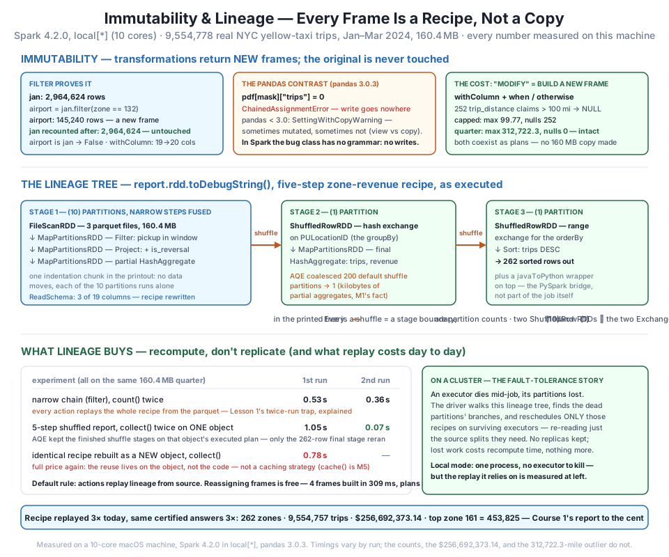
jan (2,964,624 rows) filtered to airport (145,240) and recounted unchanged; pandas 3.0.3's ChainedAssignmentError marks the aliasing-bug class Spark structurally lacks; the immutable "modify" (withColumn + when) nulled 252 dirty distances in capped while quarter kept its 312,722.3-mile absurdity intact. Middle: the real toDebugString tree of the five-step report — FileScanRDD over 3 files in 10 partitions, two ShuffledRowRDD boundaries (AQE coalescing 200→1), three stages, matching explain()'s two Exchanges. Bottom: what the recipe costs and buys — a narrow chain pays per action (0.53 s / 0.36 s), the same object's finished shuffle stages rerun in 0.07 s, an identical recipe rebuilt pays 0.78 s full price; and the replayed recipe reproduced Course 1's report exactly: 262 zones, 9,554,757 trips, $256,692,373.14.spark.stop()
print("session stopped")session stoppedExercise 1 — Quarantine without touching the source. Course 1’s quarter report quarantined exactly 21 stray-timestamp rows. Reproduce that number the immutable way: build a new frame from quarter with a boolean column is_stray that is True when the pickup time falls outside the window (before 2024-01-01 or on/after 2024-04-01), count the flagged rows, and then prove the operation left quarter untouched — same row count, same 19 columns, no is_stray.
Hint
withColumn("is_stray", (F.col("tpep_pickup_datetime") < "2024-01-01") | (F.col("tpep_pickup_datetime") >= "2024-04-01")) builds the flag; .filter(F.col("is_stray")).count() should return exactly 21. For the untouched-source proof, len(quarter.columns) and "is_stray" in quarter.columns settle it without running a single job — the schema is part of the plan, so checking it is free. If you get 56 instead of 21, you’ve tested per-file month bounds rather than quarter bounds — the distinction Module 1 made with the 35 month-boundary spill rows.
Exercise 2 — Predict a tree, then print it. Build (don’t run) this pipeline: filter quarter to JFK pickups (PULocationID == 132), group by DOLocationID, count, and order by count descending. From what you know — one groupBy, one orderBy — predict how many ShuffledRowRDD entries and how many indentation chunks its toDebugString tree will show, and check your prediction against explain()’s Exchange count first. Then run an action and print the tree. Do the partition numbers in parentheses match the module’s established facts?
Hint
The structure should be a twin of the lesson’s: two Exchanges in the plan (hash for the groupBy, range for the sort), therefore two ShuffledRowRDDs and three chunks in the tree, with (10) on the scan chunk. Remember the callout: under AQE, calling .rdd before any action will itself trigger the shuffle stages — run your action first if you want the printed tree to describe an execution you’ve already paid for. Top of the result, from ground truth: JFK’s most common destination is within the airport’s own zone catchment area? Check what you find against intuition — long-haul drop-offs like Midtown should dominate.
Exercise 3 — Count the replays. Take the narrow frame in_window and run three different actions on it in sequence — count(), first(), and show(3) — timing each. Then answer precisely: how many times was the 160.4 MB scan-plus-filter recipe replayed in total, and how do you know? Finally, predict (without running it) what would change if in_window had a groupBy in it, and why that still wouldn’t be a substitute for cache().
Hint
Three actions on a narrow frame = three full replays — every timing should be the same order of magnitude as the lesson’s 0.53 s count (though first() can be quicker: it only needs the first partition to produce a row, so Spark may stop early — replay doesn’t always mean complete replay). With a shuffle in the chain, the second and third actions could reuse the AQE-materialized stages only if Spark considers them the same query execution on the same object — different actions build different plans, so don’t count on it. The dependable statement is the lesson’s: actions replay lineage by default; cache() (Module 5) is the explicit, portable fix.
This lesson demonstrated Spark’s most un-pandas-like property and then priced both sides of it. Immutability, shown not asserted: filtering jan (2,964,624 rows) to airport (145,240 — Course 1’s exact January JFK count) left jan recounting to 2,964,624, airport is jan returning False, and withColumn handing back a 20-column frame while its 19-column source stood untouched. pandas 3.0.3 made the contrast vivid with a real ChainedAssignmentError — the descendant of SettingWithCopyWarning, the aliasing-bug class that Spark’s no-write grammar makes unwritable — and copy-on-write showed pandas itself migrating toward Spark’s discipline. The cost is that “modify” means “rebuild”: withColumn + when/otherwise nulled the quarter’s 252 implausible trip_distance values (max 312,722.3 mi) into a new capped frame in which the max is 99.77, with the original at zero nulls. The purchase is lineage: five frames built in 309 ms as plans, explain() growing step by step (with PushedFilters and a three-column ReadSchema proving the optimizer rewrites the recipe), and the real toDebugString tree — FileScanRDD at (10) partitions, two ShuffledRowRDD stage boundaries, AQE’s 200→1 coalescing — as the structure a cluster walks to recompute lost partitions instead of replicating data. Recomputation measured for real: a narrow count paid twice (0.53 s / 0.36 s), the same report object re-collected in 0.07 s (AQE stage reuse — object-bound, not a caching strategy), an identical rebuilt recipe paid 0.78 s full price, and the report cross-checked Course 1 to the cent: 262 zones, 9,554,757 trips, $256,692,373.14, podium 161/237/132 exact — with the window’s 115,894 reversals versus the files’ 115,895 tracing to a single quarantined stray.
SettingWithCopyWarning class) have no grammar to occur in.withColumn + when/otherwise producing a new frame (reusing a column name replaces that column); the source frame remains bit-for-bit intact, and both frames coexist as plans, not copies.cache() addresses explicitly; AQE’s reuse of finished shuffle stages on the same object (1.05 s → 0.07 s) vanishes for an identical recipe in a new object (0.78 s) and must not be mistaken for caching.CityFlow’s Spark pipelines are headed for scheduled scripts that run unattended at 3 a.m., and immutability plus lineage is why they can be trusted there. The pandas habits this lesson retired — mutate in place, hope the slice was a view, rerun the notebook top-to-bottom when state gets confused — are habits of interactive work, where a human is present to notice that a frame isn’t what it was. A production pipeline has no such human. Spark’s guarantee that no step can silently change a frame another step depends on is what makes a 40-transformation job debuggable: every intermediate is exactly what its recipe says, every time, and the recipe itself (explain(), toDebugString) is printable evidence you can attach to a code review. The same property carried the audit: this lesson’s report replayed its recipe three separate times and produced $256,692,373.14 all three times, to the cent, against Course 1’s independently-computed ground truth — reproducibility isn’t a virtue the team practices, it’s a property the engine enforces. And the judgment half matters just as much: knowing that lineage replay is real work (0.53 s per action here; hours on a production-sized chain) tells you when the constraint bites and when to reach for Module 5’s cache() — deliberately, not by leaning on an AQE artifact that evaporates the next time the script builds its frames fresh. Engineers who understand that frames are recipes stop asking “where is my data?” and start asking “is my recipe right?” — and that question has a printable answer.
You now hold all four pieces of Module 2 separately: the behavioural rule (transformations plan, actions pay), the substrate (RDDs and their partitions), the execution anatomy (jobs, stages, tasks, and what AQE does to them), and — as of today — the conceptual foundation underneath all of it (immutable frames whose lineage makes every result recomputable and every plan rewritable). What you have not yet done is use all four at once, on one job, the way you will every working day from now on. Lesson 5, Guided Project: Trace One Job, is exactly that: take a single real aggregation over the quarter — one with known, Course-1-certified answers — and walk it end to end. You will time the lazy build, annotate the explain() plan operator by operator, write down predictions — how many jobs, how many stages, how many tasks, where the shuffles fall — before touching an action, then execute and hold your predictions up against what statusTracker and the Spark UI actually report, AQE surprises included. The deliverable is a read-one-job checklist you can reuse on any Spark job you ever meet cold. Prediction before execution is the discipline that separates engineers who understand their engine from engineers who watch it; Lesson 5 is where you prove you’re the first kind.
Keep DATATWEETS free. Help fund practical data, AI, and engineering lessons for learners worldwide.
