Title here
Summary here
Module 2 handed you four lenses for the same engine. Lesson 1 showed that transformations build a plan while actions pay for it; Lesson 2 went underneath to the RDD and measured why opaque Python lambdas lose to a plan Catalyst can read; Lesson 3 named the execution hierarchy — one action becomes jobs, jobs split into stages at shuffles, stages fan out into one task per partition; Lesson 4 explained why every transformation returns a new DataFrame and how lineage makes recomputation, not replication, Spark’s fault-tolerance story. Each lesson used the lenses one at a time. This project uses all four at once, on one job, and holds the result to a standard no demo can fake: prediction before execution.
Here is the wager. If Module 2 actually taught you how Spark thinks, you should be able to take one real aggregation — CityFlow’s per-zone trip counts and revenue for the quarter window, an answer Course 1 established to the cent — and call its shot: how many jobs the one collect() will spawn, how many stages, how many tasks, which stage gets skipped, what AQE will quietly rewrite. Written down, before running, in numbers. Then the status tracker reports what actually happened, and every prediction gets scored HELD or MISSED — and the misses get explained, because a miss you can explain is worth more than a guess that happens to land. The answer itself gets the same treatment: the window must keep exactly 9,554,757 trips worth exactly $256,692,373.14, or the trace was a tour of a broken job.
By the end of this project, you will be able to:
explain() plan bottom-up and extract the facts that determine execution shape: pushed filters, pruned columns, and the ExchangesetJobGroup and statusTracker() and score every prediction against realityYou’ll need pyspark (with the Java 17/21 runtime from the course setup page) — everything else is the Python standard library.
Six criteria define “done” for this trace, and they are deliberately harsher than “the numbers came out right”:
explain() alone: which columns the scan reads, which filters got pushed into it, where the partial and final aggregates sit, and where the one shuffle lives.statusTracker() supplies the real jobs, stages, and task counts; every prediction is scored HELD or MISSED, and every MISS gets a real explanation.The data is the same quarter as always — New York City’s public-domain Yellow Taxi trip records from the NYC Taxi & Limousine Commission, plus the zone lookup:
https://d37ci6vzurychx.cloudfront.net/trip-data/yellow_tripdata_2024-01.parquet (2,964,624 rows, 48 MB)https://d37ci6vzurychx.cloudfront.net/trip-data/yellow_tripdata_2024-02.parquet (3,007,526 rows, 48 MB)https://d37ci6vzurychx.cloudfront.net/trip-data/yellow_tripdata_2024-03.parquet (3,582,628 rows, 57 MB)https://datatweets.com/datasets/nyc-taxi/taxi_zone_lookup.csv (265 zones)Download once, then every block below reads the local copies:
# gate: skip
# Fetch once; all later blocks read the local cached copies by name.
import urllib.request
for m in ("01", "02", "03"):
    urllib.request.urlretrieve(
        f"https://d37ci6vzurychx.cloudfront.net/trip-data/yellow_tripdata_2024-{m}.parquet",
        f"yellow_tripdata_2024-{m}.parquet")
urllib.request.urlretrieve(
    "https://datatweets.com/datasets/nyc-taxi/taxi_zone_lookup.csv",
    "taxi_zone_lookup.csv")
One session for the whole trace, with the status tracker in hand from the start — this project’s entire instrument panel is sc.statusTracker(), exactly as Lesson 3 used it:
import warnings; warnings.filterwarnings("ignore")
import time
from pyspark.sql import SparkSession
from pyspark.sql import functions as F

t0 = time.perf_counter()
spark = (SparkSession.builder
         .appName("cityflow")
         .master("local[*]")
         .config("spark.ui.showConsoleProgress", "false")
         .getOrCreate())
spark.sparkContext.setLogLevel("ERROR")
sc = spark.sparkContext
tracker = sc.statusTracker()
print(f"SparkSession up in {time.perf_counter() - t0:.1f} s (Spark {spark.version})")
SparkSession up in 6.2 s (Spark 4.2.0)The aggregation under trace is the smallest job that still exercises everything Module 2 taught: read the quarter, keep the window, group by pickup zone, count trips and sum revenue. One wide operation, one shuffle, one known answer. Build it with the stopwatch running — the read timed separately from the transformation chain, because Lesson 1 taught they are not the same kind of cheap:
PATHS = [f"yellow_tripdata_2024-{m:02d}.parquet" for m in (1, 2, 3)]

t0 = time.perf_counter()
trips = spark.read.parquet(*PATHS)
t_read = time.perf_counter() - t0

t0 = time.perf_counter()
report = (trips
          .where((F.col("tpep_pickup_datetime") >= "2024-01-01") &
                 (F.col("tpep_pickup_datetime") < "2024-04-01"))
          .groupBy("PULocationID")
          .agg(F.count("*").alias("trips"),
               F.sum("total_amount").alias("revenue")))
t_chain = time.perf_counter() - t0

print(f"read.parquet (3 files)      : {t_read:.2f} s")
print(f"filter -> groupBy -> agg    : {t_chain * 1000:.1f} ms")
print(f"jobs run so far             : {sorted(tracker.getJobIdsForGroup())}")
read.parquet (3 files) : 1.83 s
filter -> groupBy -> agg : 235.8 ms
jobs run so far : [0]The transformation chain — a filter over 9.5 million rows, a grouping, two aggregates — cost 236 milliseconds, and every one of those milliseconds went into building plan objects, not touching trips. That’s Lesson 1’s core fact holding at full pipeline scale. But the last line has a surprise in it: the job list is not empty. Something already ran, and this project promised to explain everything on the tracker. So, before going further — what is job 0?
for sid in tracker.getJobInfo(0).stageIds:
    si = tracker.getStageInfo(sid)
    print(f"job 0, stage {sid}: '{si.name.split(' at ')[0]}' -- "
          f"{si.numTasks} task, {si.numCompletedTasks} completed")
job 0, stage 0: 'parquet' -- 1 task, 1 completedOne stage, one task, named parquet — launched by spark.read.parquet itself. This is the 1.83 s read explained: Spark ran a single tiny task to open the file footers and confirm the three schemas agree, because with multiple files even schema-checking is work it delegates to the engine. Module 1 said the read touches “footers only” — here is that footer touch, showing up as an actual job with an actual task. Zero of the 9,554,778 trips have moved.
Lazy is not zero I/O
“Transformations run nothing” is the right model with one asterisk, and job 0 is the asterisk. spark.read.parquet must know the schema at build time — every transformation you chain afterwards is validated against it — so it reads the file footers, and with several files it may launch a small 1-task job to do it. The rows stay untouched. When you trace your own jobs and find one you never asked for, check its name and task count before assuming your pipeline executed early: a 1-task parquet job is the price of a schema, not a scan.
Everything Spark intends to do is already written down — explain() prints it. Lesson 1 read these plans for the vocabulary and Module 4 will dissect them line by line; here the job is extraction: pull out exactly the facts that determine the execution shape.
report.explain()== Physical Plan ==
AdaptiveSparkPlan isFinalPlan=false
+- HashAggregate(keys=[PULocationID#7], functions=[count(1), sum(total_amount#16)])
+- Exchange hashpartitioning(PULocationID#7, 200), ENSURE_REQUIREMENTS, [plan_id=15]
+- HashAggregate(keys=[PULocationID#7], functions=[partial_count(1), partial_sum(total_amount#16)])
+- Project [PULocationID#7, total_amount#16]
+- Filter ((isnotnull(tpep_pickup_datetime#1) AND (tpep_pickup_datetime#1 >= 2024-01-01 00:00:00)) AND (tpep_pickup_datetime#1 < 2024-04-01 00:00:00))
+- FileScan parquet [tpep_pickup_datetime#1,PULocationID#7,total_amount#16] Batched: true,
PushedFilters: [IsNotNull(tpep_pickup_datetime),
GreaterThanOrEqual(tpep_pickup_datetime,2024-01-01T00:00),
LessThan(tpep_pickup_datetime,2024-04-01T00:00)],
ReadSchema: struct<tpep_pickup_datetime:timestamp_ntz,PULocationID:int,total_amount:double>(the FileScan line is wrapped and its file paths elided to fit the page; DataFilters and Location fields trimmed)
Read it bottom-up — the bottom is where execution starts — and take four facts:
ReadSchema lists three columns out of the nineteen in the file: the timestamp, the zone, the money. Catalyst pruned the other sixteen — this is precisely the pruning Lesson 2 showed the RDD path losing, because no optimizer can see inside a Python lambda. And PushedFilters carries the window bounds into the scan itself: rows outside the quarter are discarded at read time, not in a later step.Filter, Project, and the first HashAggregate all consume their input partition-by-partition with no data movement — Lesson 3’s narrow transformations. They will run inside the same stage as the scan.partial_count / partial_sum below the Exchange, count / sum above it: each input partition pre-aggregates its own rows down to its own zone subtotals, and only those subtotals cross the shuffle. Nine and a half million rows go in; a few hundred subtotal rows per partition come out.Exchange. hashpartitioning(PULocationID, 200) — the one point where data must move between partitions so that each zone’s subtotals land in one place. One Exchange means one shuffle means one stage boundary. And the wrapper says AdaptiveSparkPlan isFinalPlan=false: this plan is a draft, and AQE reserves the right to rewrite it while it runs — with 200 declared shuffle partitions as the number to watch.This is the step that separates a trace from a tour. Everything needed to call the shot is on the table; the one plan-level fact still missing is how many partitions the scan will use, and Lesson 3 showed that’s plan metadata, readable without executing anything:
print(f"scan partitions planned : {trips.rdd.getNumPartitions()}")
print(f"defaultParallelism      : {sc.defaultParallelism}")
print(f"jobs run so far         : {sorted(tracker.getJobIdsForGroup())}")
scan partitions planned : 10
defaultParallelism : 10
jobs run so far : [0]Ten partitions for the full 160 MB quarter — the same number Module 1 measured for January alone, because the planner splits whatever bytes it’s given to feed ten cores; and still only job 0 on the books, so the partition count really is plan metadata, not a dress rehearsal. Now the predictions, reasoned from Module 2’s facts and committed to a dict so the scoring later is mechanical:
collect() do exactly this.count() cost 3.25 s; this job reads three columns instead of zero but aggregates as it goes. Somewhere in that neighbourhood.PREDICTED = {
"jobs": 2,
"map-stage tasks": 10,
"final-stage tasks": 1,
"tasks scheduled": 21,
"tasks actually run": 11,
}
PREDICTED_SECONDS = (2.0, 4.0)
for k, v in PREDICTED.items():
print(f" predicted {k:<18}: {v}")
print(f" predicted wall time : {PREDICTED_SECONDS[0]:.0f}-{PREDICTED_SECONDS[1]:.0f} s") predicted jobs : 2
predicted map-stage tasks : 10
predicted final-stage tasks : 1
predicted tasks scheduled : 21
predicted tasks actually run: 11
predicted wall time : 2-4 sThose five numbers and one range were written before the action ran, and nothing after this point may edit them. That’s the whole discipline: a prediction you can revise after seeing the answer is a caption, not a prediction.
One action, wrapped in its own job group so the tracker can report exactly what this collect() caused and nothing else — the same isolation trick as Lesson 3:
sc.setJobGroup("trace", "per-zone quarter counts + revenue")
t0 = time.perf_counter()
zone_rows = report.collect()
t_run = time.perf_counter() - t0
sc.setJobGroup(None, None)

print(f"collect() returned {len(zone_rows)} zone rows in {t_run:.2f} s\n")

job_ids = sorted(tracker.getJobIdsForGroup("trace"))
stages = []
for jid in job_ids:
    print(f"job {jid}:")
    for sid in sorted(tracker.getJobInfo(jid).stageIds):
        si = tracker.getStageInfo(sid)
        tag = "SKIPPED -- result reused" if si.numCompletedTasks == 0 else "ran"
        print(f"  stage {sid}: {si.numTasks:>2} tasks scheduled, "
              f"{si.numCompletedTasks:>2} completed   [{tag}]")
        stages.append((jid, sid, si.numTasks, si.numCompletedTasks))
n_sched = sum(s[2] for s in stages)
n_done = sum(s[3] for s in stages)
print(f"\ntotal: {len(job_ids)} jobs, {n_sched} tasks scheduled, {n_done} actually ran")
collect() returned 262 zone rows in 1.96 s
job 1:
stage 1: 10 tasks scheduled, 10 completed [ran]
job 2:
stage 2: 10 tasks scheduled, 0 completed [SKIPPED -- result reused]
stage 3: 1 tasks scheduled, 1 completed [ran]
total: 2 jobs, 21 tasks scheduled, 11 actually ranThere is the whole anatomy, exactly as Lesson 3 drew it: job 1 is AQE materializing the shuffle’s map side — ten tasks, one per scan partition, each running the fused scan-filter-partial-aggregate and writing its zone subtotals as shuffle output. Job 2 re-lists that map stage (ten tasks scheduled, zero run — skipped, its output already sitting in shuffle files) and then runs the finish as a single task, because AQE looked at the actual shuffle payload and collapsed 200 planned partitions into one. Nine and a half million rows in, 262 rows out, eleven tasks of real work.
First, catch AQE in writing. The same explain() that printed a draft in Step 2 prints the as-built plan now that the query has run:
report.explain()== Physical Plan ==
AdaptiveSparkPlan isFinalPlan=true
+- == Final Plan ==
ResultQueryStage 1
+- *(2) HashAggregate(keys=[PULocationID#7], functions=[count(1), sum(total_amount#16)])
+- AQEShuffleRead coalesced
+- ShuffleQueryStage 0
+- Exchange hashpartitioning(PULocationID#7, 200), ENSURE_REQUIREMENTS, [plan_id=44]
+- *(1) HashAggregate(keys=[PULocationID#7], functions=[partial_count(1), partial_sum(total_amount#16)])
+- *(1) Project [PULocationID#7, total_amount#16]
+- *(1) Filter (...)
+- *(1) ColumnarToRow
+- FileScan parquet [tpep_pickup_datetime#1,PULocationID#7,total_amount#16] ...
+- == Initial Plan ==
(the Step 2 draft, unchanged -- omitted here)(filter condition and FileScan details elided — they are identical to Step 2’s plan)
isFinalPlan=true now, and the rewrite is legible: the query was cut at the Exchange into ShuffleQueryStage 0 (job 1) and ResultQueryStage 1 (job 2), and between them sits AQEShuffleRead coalesced — the written confession for the 200→1 collapse the task counts showed. The *(1) and *(2) markers even label the two fused code regions, one per stage. Now the scoring, mechanical, straight from the dict:
actual = {
    "jobs": len(job_ids),
    "map-stage tasks": stages[0][3],
    "final-stage tasks": stages[-1][3],
    "tasks scheduled": n_sched,
    "tasks actually run": n_done,
}
print(f"  {'prediction':<20} {'predicted':>9} {'actual':>9}   verdict")
for k in PREDICTED:
    verdict = "HELD" if PREDICTED[k] == actual[k] else "MISSED"
    print(f"  {k:<20} {PREDICTED[k]:>9} {actual[k]:>9}   {verdict}")
lo, hi = PREDICTED_SECONDS
t_verdict = "HELD" if lo <= t_run <= hi else "MISSED"
print(f"  {'wall time':<20} {f'{lo:.0f}-{hi:.0f} s':>9} {f'{t_run:.2f} s':>9}   {t_verdict}")
prediction predicted actual verdict
jobs 2 2 HELD
map-stage tasks 10 10 HELD
final-stage tasks 1 1 HELD
tasks scheduled 21 21 HELD
tasks actually run 11 11 HELD
wall time 2-4 s 1.96 s MISSEDFive HELD, one MISSED — and the miss is the most instructive row on the page. Every structural prediction held exactly, because structure is determined by things Module 2 taught you to read: the plan’s one Exchange, the scan’s 10 partitions, AQE’s materialize-then-finish rhythm. Those are deterministic. Wall time is not — and this prediction didn’t just miss, it missed in both directions. When this project was first executed while being written, on a cold file cache, the same collect() took 7.97 s — double the top of the predicted band. The run pasted above, made moments later with all 160 MB already sitting in the operating system’s page cache, took 1.96 s — under the bottom of it. Identical plan, identical 11 tasks, a 4× wall-time spread, and none of it was Spark’s decision: the variable that dominated was whether the bytes came from disk or from RAM the OS had already cached. That’s the honest boundary of this module’s predictive power. Learn the plan and the hierarchy and you can call jobs, stages, and tasks to the digit; the clock belongs to the machine’s state, which is why engineers profile the shape of a job to understand it and trust only repeated measurements for its speed.
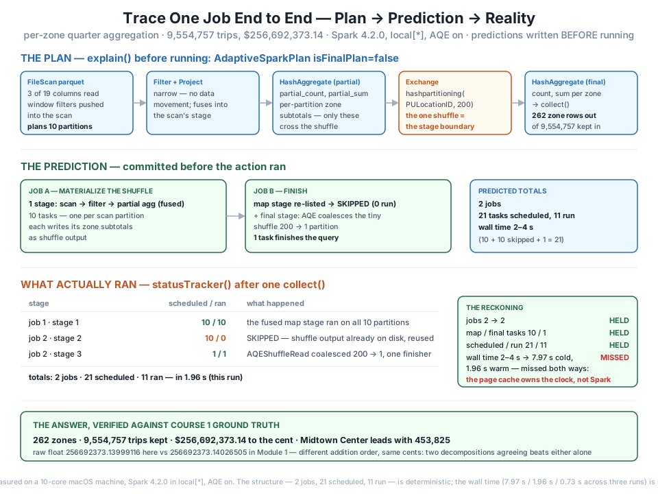
Exchange — so the predictions (middle), written before running, call 2 jobs, a 10-task map stage, a skipped re-list, and an AQE-coalesced 1-task finish: 21 scheduled, 11 run. The status tracker (bottom) confirms every structural call — 5 of 6 predictions HELD — while wall time missed in both directions (predicted 2–4 s; 7.97 s cold cache, 1.96 s warm), because the page cache, not Spark, owns the clock. The answer lands on Course 1's ground truth exactly: 9,554,757 trips, $256,692,373.14 to the cent.A perfectly traced job computing the wrong thing is worse than useless — it’s convincing. Course 1’s zone-hour report is the answer key: the quarter window keeps 9,554,757 trips worth $256,692,373.14, and the top five zones are known to the trip. The 262 collected rows carry zone IDs; the names come from the lookup CSV via plain Python, deliberately outside Spark so the traced job stays exactly the two jobs already on the books — and keyed on LocationID, never on the name, because two different zones are both called “Corona”:
import csv
with open("taxi_zone_lookup.csv") as f:
    zone_names = {int(r["LocationID"]): r["Zone"] for r in csv.DictReader(f)}

GROUND = {"trips": 9_554_757, "revenue": "256,692,373.14",
          "top5": [(161, 453_825), (237, 439_138), (132, 429_745),
                   (236, 416_508), (162, 336_460)]}

kept = sum(r["trips"] for r in zone_rows)
revenue = sum(r["revenue"] for r in zone_rows)
rev_str = f"{revenue:,.2f}"
print(f"zones in the result : {len(zone_rows)}")
print(f"trips kept          : {kept:,}   expected {GROUND['trips']:,}   "
      f"{'OK' if kept == GROUND['trips'] else 'MISMATCH'}")
print(f"revenue raw float   : {revenue!r}")
print(f"revenue             : ${rev_str}   expected ${GROUND['revenue']}   "
      f"{'OK' if rev_str == GROUND['revenue'] else 'MISMATCH'}")
print("busiest zones:")
top5 = sorted(zone_rows, key=lambda r: r["trips"], reverse=True)[:5]
for r, (exp_id, exp_n) in zip(top5, GROUND["top5"]):
    ok = "OK" if (r["PULocationID"], r["trips"]) == (exp_id, exp_n) else "MISMATCH"
    print(f"  {zone_names[r['PULocationID']]:<22} {r['trips']:>8,}   "
          f"expected {exp_n:>8,}   {ok}")
zones in the result : 262
trips kept : 9,554,757 expected 9,554,757 OK
revenue raw float : 256692373.13999116
revenue : $256,692,373.14 expected $256,692,373.14 OK
busiest zones:
Midtown Center 453,825 expected 453,825 OK
Upper East Side South 439,138 expected 439,138 OK
JFK Airport 429,745 expected 429,745 OK
Upper East Side North 416,508 expected 416,508 OK
Midtown East 336,460 expected 336,460 OKEvery check passes: the trip count exactly, the top five to the digit, the revenue to the cent. The job whose execution you just predicted stage-by-stage is also correct — the two halves of trust, welded. And the raw float deserves one more look, because it quietly confirms Lesson 4’s immutability story from an unexpected angle: this run’s raw sum is 256692373.13999116, while Module 1’s project — summing the same window as one Spark aggregate instead of 262 per-zone subtotals added in Python — got 256692373.14026505. Different grouping, different addition order, different last bits; identical cents after rounding. Two independent decompositions of the same quarter agreeing to the cent is a stronger verification than either number alone.
Same data, different last bits
Float64 addition is not associative, so how a computation is decomposed leaves fingerprints in the last bits: summing 9,554,757 doubles in one pass and summing 262 zone subtotals produce raw values that differ by a quarter of a milli-cent here. Neither is “the” true value — both are honest float64 renderings of it. This is why the course’s ground-truth checks compare formatted currency, never raw floats, and why a checker that demands bit-identical floats across two engines (or two groupings) is testing the decomposition, not the data.
The numbers above expire with this dataset; the procedure doesn’t. This is the deliverable CityFlow keeps — first the checklist, which is nothing more than the seven steps you just executed, compressed to what you actually do at a terminal with an unfamiliar job:
READ ONE JOB -- the checklist
==============================
BEFORE RUNNING
 1. Time the build. Transformations should return in ms.
    Anything slower is already executing -- find out what (a 1-task
    'parquet' footer job is normal; a full scan is not).
 2. explain(). Read bottom-up. Extract:
      - ReadSchema: which columns survive pruning?
      - PushedFilters: which predicates reach the scan?
      - Count the Exchanges: each one is a shuffle = a stage boundary.
      - AdaptiveSparkPlan isFinalPlan=false? Then AQE will re-shape it.
 3. df.rdd.getNumPartitions() on the scan -> tasks in the first stage.
    (Plan metadata -- costs no job.)
 4. WRITE THE PREDICTIONS DOWN: jobs, tasks per stage, scheduled vs
    run, wall time. With AQE expect: one materialization job per
    shuffle, re-listed stages skipped, tiny shuffles coalesced to 1.
RUN
 5. setJobGroup() around the ONE action, then statusTracker():
    jobs -> stages -> numTasks vs numCompletedTasks
    (scheduled-but-0-completed = skipped = reused shuffle output).
 6. explain() again. isFinalPlan=true shows what AQE actually did
    (AQEShuffleRead coalesced, ShuffleQueryStage / ResultQueryStage).
AFTER
 7. Score every prediction HELD or MISSED, and explain the misses.
    Structure misses mean your model of the plan is wrong -- stop and
    fix that before touching performance.
 8. Verify the ANSWER against something independent. A beautifully
    traced wrong answer is still wrong.
And the traced script — the same trace as a re-runnable file, with the predictions derived from the plan probe instead of hard-coded, so it keeps working when the partition count changes (as Module 1 proved it does under local[2]):
"""cityflow_trace_job.py -- trace one Spark job end to end.

Reusable shape: build lazily, read the plan, write predictions down,
execute under a job group, pull the real jobs/stages/tasks from the
status tracker, and verify the answer against independent ground truth.
"""
import time
import uuid
import warnings; warnings.filterwarnings("ignore")
from pyspark.sql import SparkSession
from pyspark.sql import functions as F

WINDOW = ("2024-01-01", "2024-04-01")
GROUND2 = {"trips": 9_554_757, "revenue": "256,692,373.14"}


def get_session():
    spark = (SparkSession.builder
             .appName("cityflow")
             .master("local[*]")
             .config("spark.ui.showConsoleProgress", "false")
             .getOrCreate())
    spark.sparkContext.setLogLevel("ERROR")
    return spark


def build_pipeline(spark):
    """The lazy build. Returns the un-executed frame plus the build time."""
    t0 = time.perf_counter()
    trips = spark.read.parquet(*[f"yellow_tripdata_2024-{m:02d}.parquet"
                                 for m in (1, 2, 3)])
    pipe = (trips
            .where((F.col("tpep_pickup_datetime") >= WINDOW[0]) &
                   (F.col("tpep_pickup_datetime") < WINDOW[1]))
            .groupBy("PULocationID")
            .agg(F.count("*").alias("trips"),
                 F.sum("total_amount").alias("revenue")))
    return pipe, trips.rdd.getNumPartitions(), time.perf_counter() - t0


def execute_traced(spark, pipe):
    """Run ONE action under its own job group; return rows + the real shape."""
    sc = spark.sparkContext
    group = f"trace-{uuid.uuid4().hex[:8]}"      # unique per run
    sc.setJobGroup(group, "traced action")
    t0 = time.perf_counter()
    rows = pipe.collect()
    elapsed = time.perf_counter() - t0
    sc.setJobGroup(None, None)

    tracker = sc.statusTracker()
    shape = []
    for jid in sorted(tracker.getJobIdsForGroup(group)):
        for sid in sorted(tracker.getJobInfo(jid).stageIds):
            si = tracker.getStageInfo(sid)
            shape.append((jid, sid, si.numTasks, si.numCompletedTasks))
    return rows, shape, elapsed


def main():
    spark = get_session()
    pipe, n_scan, t_build = build_pipeline(spark)

    predicted = {"jobs": 2, "tasks scheduled": 2 * n_scan + 1,
                 "tasks run": n_scan + 1}
    rows, shape, elapsed = execute_traced(spark, pipe)
    actual = {"jobs": len({s[0] for s in shape}),
              "tasks scheduled": sum(s[2] for s in shape),
              "tasks run": sum(s[3] for s in shape)}

    kept = sum(r["trips"] for r in rows)
    rev = f"{sum(r['revenue'] for r in rows):,.2f}"

    print("TRACE -- per-zone quarter aggregation")
    print(f"  built lazily in {t_build:.2f} s; scan plans {n_scan} partitions")
    for jid, sid, sched, done in shape:
        tag = "SKIPPED" if done == 0 else "ran"
        print(f"  job {jid} stage {sid}: {sched:>2} scheduled / {done:>2} ran  [{tag}]")
    checks = []
    for k in predicted:
        ok = predicted[k] == actual[k]
        checks.append(ok)
        print(f"  {k:<16} predicted {predicted[k]:>2}, actual {actual[k]:>2}  "
              f"{'[OK]' if ok else '[MISS]'}")
    for label, got, want in [("trips kept", f"{kept:,}", f"{GROUND2['trips']:,}"),
                             ("revenue", f"${rev}", f"${GROUND2['revenue']}")]:
        ok = got == want
        checks.append(ok)
        print(f"  {label:<16} {got}  vs ground truth {want}  "
              f"{'[OK]' if ok else '[MISMATCH]'}")
    print(f"  executed in {elapsed:.2f} s -- "
          f"{sum(checks)} of {len(checks)} checks passed")
    spark.stop()


if __name__ == "__main__":
    main()
TRACE -- per-zone quarter aggregation
built lazily in 0.17 s; scan plans 10 partitions
job 4 stage 5: 10 scheduled / 10 ran [ran]
job 5 stage 6: 10 scheduled / 0 ran [SKIPPED]
job 5 stage 7: 1 scheduled / 1 ran [ran]
jobs predicted 2, actual 2 [OK]
tasks scheduled predicted 21, actual 21 [OK]
tasks run predicted 11, actual 11 [OK]
trips kept 9,554,757 vs ground truth 9,554,757 [OK]
revenue $256,692,373.14 vs ground truth $256,692,373.14 [OK]
executed in 0.73 s -- 5 of 5 checks passedRun inside the still-warm session, the script’s job IDs continue from where the lesson left off (jobs 4 and 5 — its own footer read claimed job 3), its build takes 0.17 s now that the footers are cached, and the execution itself drops to 0.73 s — a third data point on the wall-time spread, and further proof that the eleven tasks are the invariant while the clock is weather. Five checks, five [OK]s, and spark.stop() closes the session the project opened.
These extend the trace. Each one is a prediction exercise first and a coding exercise second — write the numbers down before you run.
Exercise 1 — Re-trace under local[2]. Module 1 established that a local[2] session plans the same quarter read as 3 partitions instead of 10 — the plan follows the cores. Predict the complete trace shape for this exact aggregation under local[2] — jobs, tasks per stage, scheduled versus run — then build the session and verify with the same instrumentation. The answer (9,554,757 trips, $256,692,373.14) must not move.
Hint
The master is fixed when a session is created, so spark.stop() first and build a fresh one with .master(“local[2]”). Derive the shape from the rule, not from memory: 3 scan partitions → a 3-task map stage; AQE still materializes the shuffle as its own job and still coalesces the tiny finish to 1 task → 2 jobs, scheduled, run. If your prediction for scheduled tasks misses, check whether you remembered the skipped re-listing of the map stage — forgetting it is the most common way to be wrong by exactly one stage’s worth of tasks.
Exercise 2 — Add a sort, gain a shuffle. Append .orderBy(F.desc("trips")) to the aggregation and read the new explain() before running. Predict what the plan gains, what the trace gains, and whether the coalesced-to-1 pattern repeats — then execute under a fresh job group and score yourself.
Hint
Count the Exchanges: orderBy is a wide transformation, so the plan gains a second Exchange — rangepartitioning this time, because a global sort needs range boundaries, and Spark samples the data to find them. Expect the trace to gain roughly one job (AQE materializes each shuffle before planning past it), and expect the sort stage over 262 rows to be coalesced just like the aggregation’s finish was. The deeper lesson to look for: the map stage from the first shuffle shows up re-listed and skipped again — shuffle output is the currency stages trade in.
Exercise 3 — The twice-run trap, measured in tasks. Lesson 1 showed that two actions on one lazy frame execute the whole pipeline twice; now you can weigh that in tasks instead of seconds. Predict what the job group will contain if you run report.collect() twice back-to-back — jobs, scheduled, run — then do it under one job group and check.
Hint
Each action starts a fresh query execution, and Lesson 4’s lineage story tells you what that means: nothing is remembered, everything is recomputed from source. Expect an exact structural copy — 2 more jobs, 21 more scheduled, 11 more run, so in total — including a second 10-task scan of all 160 MB. The skipped-stage reuse you saw inside one action does not carry across actions: shuffle output is reused within a query, not between queries. The fix for that is caching, which is exactly where Module 5 picks up — you now have the before-picture in task counts.
You traced one real job through everything Module 2 taught, and the trace held. The pipeline — read the quarter, filter the window, group 9.5 million trips by zone, count and sum — was built lazily in 236 ms, with the only job on the books a 1-task parquet footer read that spark.read.parquet ran to get its schema. The plan, read before execution, fixed the structure: a 3-of-19-column scan with the window bounds pushed into it, narrow steps fused, the aggregation split into partial and final halves around exactly one Exchange (hashpartitioning(PULocationID, 200)), all under isFinalPlan=false. The predictions, written down before the action and reasoned from the module’s facts — 10 scan partitions, AQE’s materialize-then-finish rhythm, tiny shuffles coalesced — called 2 jobs, a 10-task map stage, a 1-task finish, 21 tasks scheduled, 11 run, and the status tracker confirmed every one: five HELD. The single MISS was wall time, and it missed in both directions — 7.97 s on the first cold-cache execution, 1.96 s on the warm re-run, against a 2-4 s prediction — because the OS page cache, not Spark, owns the clock; the post-run plan (isFinalPlan=true, AQEShuffleRead coalesced) put AQE’s 200→1 rewrite in writing. The answer matched Course 1’s ground truth exactly — 262 zones, 9,554,757 trips, $256,692,373.14 to the cent, top five zones to the digit — with this run’s raw float (256692373.13999116) differing from Module 1’s (256692373.14026505) in the last bits only, because 262 Python-summed subtotals and one Spark sum decompose the same addition differently. The method now lives in a reusable read-one-job checklist and cityflow_trace_job.py, whose re-run — 11 tasks again, 0.73 s this time — passed 5 of 5 checks.
spark.read.parquet may run a 1-task job to read schemas at build time; lazy means no rows move, not zero I/O. Check a surprise job’s name and task count before assuming early execution.isFinalPlan=true and AQEShuffleRead coalesced.The gap between engineers who use Spark and engineers who can be trusted with it is exactly the skill this project drilled: reading what the engine intends, committing to what should happen, and reconciling against what did. When a production job that ran in ten minutes yesterday takes an hour today, the untrained response is to re-run it and hope; the trained response is the checklist — did the plan change (a lost pushdown, a new Exchange), did the shape change (more tasks, a stage no longer skipped), or did only the clock change (same 11 tasks, slower machine)? Those three diagnoses have three completely different fixes, and telling them apart takes minutes with explain() and the status tracker, or days without them. Just as important is the miss this project kept honest: wall time defied a careful prediction twice, in opposite directions, on the same laptop within the same minute. Engineers who internalize that — structure is contract, timing is weather — stop chasing phantom regressions and start anchoring their debugging in the things Spark actually promises. CityFlow’s zone report now rests on a job whose every task is accounted for and whose every number matches a second, independent engine to the cent. That’s not ceremony; that’s what “verified” means.
That completes Module 2: SparkSession, RDDs & Lazy Evaluation — laziness measured behaviourally, the RDD underneath and the price of opaque lambdas, the job-stage-task hierarchy read from a live scheduler, immutability and the lineage that makes recomputation Spark’s safety net, and now one real job traced end to end with every prediction on the record.
But notice what this module took for granted: the pipeline itself was three lines — a filter, a groupBy, two aggregates. Course 1’s zone-hour report needed far more than that: window boundaries and an hourly bucketing, quarantine counts, per-zone-per-hour cells — 240,917 of them — and a defensible policy for every dirty row. You can now read any plan Spark hands you; the next step is deserving richer plans to read. Module 3 — DataFrames & Transformations — is where the API itself gets mastered: selecting and deriving columns, timestamp functions, conditional logic, joins done right, and multi-key aggregations — culminating in rebuilding the full zone-hour report in Spark and checking all 240,917 buckets against Course 1’s ground truth. The engine’s behaviour is no longer a mystery; now it’s time to speak its language fluently.
Keep DATATWEETS free. Help fund practical data, AI, and engineering lessons for learners worldwide.
