Title here
Summary here
Module 3 made you fluent in the DataFrame API — columns, filters, joins, aggregations — and you used it to rebuild CityFlow’s zone-hour report in Spark, reproducing Course 1’s audited totals on nine and a half million real trips. Along the way you kept meeting a word without ever being formally introduced to it: Catalyst, the optimizer. Every plan you read in Module 2, every Exchange and HashAggregate, was Catalyst’s doing. This module makes Catalyst the subject rather than the scenery, and it opens with a claim that surprises most engineers arriving from either pandas or SQL: the DataFrame API you just learned is not the engine. It is one of two front-ends bolted onto the same engine. The other is SQL — real, standard SELECT ... GROUP BY SQL — and the two are not merely equivalent in their answers. They compile to the same physical plan, node for node.
That is a strong claim, and this lesson’s job is to prove it rather than assert it. You’ll register CityFlow’s trips DataFrame as a temp view, write the zone-hour report a second time as a SQL string, and then put the two side by side under .explain(). The plans that come back are byte-identical except for a handful of generated node ids — and we’ll erase those with a regex to show that what remains matches exactly. Once you’ve seen that, the practical lesson follows on its own: neither dialect is faster, so you choose between them by which one reads more clearly for the task in front of you, and you mix them freely, because the result of spark.sql(...) is just a DataFrame you keep chaining. We finish with the catalog — how Spark tracks the views you register — and one honest gotcha about what a temp view actually is, which turns out to matter for Module 5.
By the end of this lesson, you will be able to:
createOrReplaceTempView and run SQL against it with spark.sql(...), understanding that the result is an ordinary DataFrame.explain() output and showing the physical plans are identical once cosmetic node ids are erasedcreateOrReplaceGlobalTempView and the global_temp database, introspect views with spark.catalog, and explain why a temp view is a named plan, not a cached tableYou’ll need pyspark with the JDK configured as in Module 1, Lesson 3, and pyspark.sql.functions as F. Start the session.
Same session shape as always — named, local, quiet. We also pull in three tools from the standard library (io, re, and redirect_stdout) that we’ll need near the end to capture and compare plan text; import them now so every later block can lean on them:
import warnings
warnings.filterwarnings("ignore")
import io, re
from contextlib import redirect_stdout

from pyspark.sql import SparkSession
from pyspark.sql import functions as F

spark = (SparkSession.builder
         .appName("cityflow")
         .master("local[*]")
         .config("spark.ui.showConsoleProgress", "false")
         .getOrCreate())
spark.sparkContext.setLogLevel("ERROR")
print("Spark", spark.version, "-", spark.sparkContext.defaultParallelism, "task slots")
Spark 4.2.0 - 10 task slotsNow read the three monthly files — a plan, so this returns instantly — and then do the one new thing this whole module builds on: register that DataFrame as a temp view named trips. A temp view is a name you attach to a DataFrame’s plan so that Spark SQL can find it by that name inside a query string. Once it exists, spark.sql("... FROM trips ...") resolves trips to exactly this plan:
months = ["yellow_tripdata_2024-01.parquet",
          "yellow_tripdata_2024-02.parquet",
          "yellow_tripdata_2024-03.parquet"]
trips = spark.read.parquet(*months)

trips.createOrReplaceTempView("trips")

sql_df = spark.sql("SELECT PULocationID, total_amount FROM trips WHERE PULocationID = 132 LIMIT 3")
print("spark.sql(...) returns a", type(sql_df).__name__)
sql_df.show()
spark.sql(...) returns a DataFrame
+------------+------------+
|PULocationID|total_amount|
+------------+------------+
| 132| 25.45|
| 132| 82.69|
| 132| 86.25|
+------------+------------+Read the first printed line before the table, because it is the quiet revelation of the lesson: spark.sql(...) returns a DataFrame — the identical type spark.read.parquet(...) handed you. It is not a special “SQL result” object, not a cursor, not a list of rows. It is a DataFrame with a plan behind it, lazy in exactly the way Module 2 taught, and everything you know how to do to a DataFrame you can do to this one. (Zone 132, by the way, is JFK Airport — those $82.69 and $86.25 fares are the flat-rate airport runs Course 1 flagged.) The name createOrReplaceTempView spells out its own semantics: it creates the view, or replaces it if a view of that name already exists, so re-running the cell is always safe.
Spark keeps a registry of these views, and you can list it through the catalog:
for t in spark.catalog.listTables():
    print(t)
Table(name='trips', catalog=None, namespace=[], description=None, tableType='TEMPORARY', isTemporary=True)One entry, trips, with tableType='TEMPORARY' and isTemporary=True. That TEMPORARY is the important word: this view lives only for the life of this SparkSession. Stop the session and it’s gone; there is no table on disk, no metadata in a metastore, nothing to clean up. We’ll come back to what “temporary” costs you at the end.
Here is the claim in concrete form. In Module 3 you built CityFlow’s zone-hour report with the DataFrame API: window to the quarter, group by pickup zone and the hour bucket, count the trips and sum the revenue. Write it again now, unchanged in spirit — this is the DataFrame API version:
report_api = (trips
    .filter((F.col("tpep_pickup_datetime") >= "2024-01-01") &
            (F.col("tpep_pickup_datetime") <  "2024-04-01"))
    .groupBy("PULocationID",
             F.date_trunc("hour", "tpep_pickup_datetime").alias("hour_bucket"))
    .agg(F.count("*").alias("trips"),
         F.round(F.sum("total_amount"), 2).alias("revenue")))

report_api.orderBy(F.col("trips").desc()).show(5, truncate=False)
+------------+-------------------+-----+--------+
|PULocationID|hour_bucket |trips|revenue |
+------------+-------------------+-----+--------+
|79 |2024-02-25 01:00:00|846 |17891.31|
|79 |2024-02-25 00:00:00|803 |17371.51|
|161 |2024-02-29 17:00:00|779 |20840.14|
|79 |2024-03-09 01:00:00|762 |15905.11|
|79 |2024-02-25 02:00:00|727 |15024.62|
+------------+-------------------+-----+--------+
only showing top 5 rowsThere is the familiar busiest bucket — zone 79 (East Village) at 2024-02-25 01:00:00 with 846 trips, the exact answer Module 3 and Course 1 verified. Now write the same report as SQL. Read the two side by side: every clause of the SQL maps to one method of the pipeline above — WHERE is the filter, GROUP BY is the groupBy, count(*) and sum(total_amount) are the agg:
report_sql = spark.sql("""
SELECT PULocationID,
date_trunc('hour', tpep_pickup_datetime) AS hour_bucket,
count(*) AS trips,
round(sum(total_amount), 2) AS revenue
FROM trips
WHERE tpep_pickup_datetime >= '2024-01-01'
AND tpep_pickup_datetime < '2024-04-01'
GROUP BY PULocationID, date_trunc('hour', tpep_pickup_datetime)
""")
print("spark.sql(...) returns a", type(report_sql).__name__)
report_sql.orderBy(F.col("trips").desc()).show(5, truncate=False)spark.sql(...) returns a DataFrame
+------------+-------------------+-----+--------+
|PULocationID|hour_bucket        |trips|revenue |
+------------+-------------------+-----+--------+
|79          |2024-02-25 01:00:00|846  |17891.31|
|79          |2024-02-25 00:00:00|803  |17371.51|
|161         |2024-02-29 17:00:00|779  |20840.14|
|79          |2024-03-09 01:00:00|762  |15905.11|
|79          |2024-02-25 02:00:00|727  |15024.62|
+------------+-------------------+-----+--------+
only showing top 5 rowsThe same five rows, to the trip and to the cent. Notice one more thing about how that table was produced: the SQL string itself has no ORDER BY — I ordered the result with report_sql.orderBy(...), a DataFrame method, called on the output of spark.sql(...). That is the “mixing” point made without ceremony. report_sql is a DataFrame, so you sort it, filter it, join it, or hand it to another function exactly as you would any DataFrame. The boundary between “SQL land” and “DataFrame land” is not a wall you cross; it doesn’t exist.
Matching answers, though, is the weak version of the claim — two different pieces of code can compute the same numbers by different routes. The strong version is that these two are not different routes at all. To show that, we have to look under both of them, at the plan.
.explain() prints the physical plan Spark will actually run. Print it for both reports and compare them line by line. (I’ve shortened the absolute Location: path to [...]; the DataFilters: and PushedFilters: lines are truncated with ... by Spark itself, not by me.)
print("=== DataFrame API plan ===")
report_api.explain()
print("=== SQL plan ===")
report_sql.explain()
=== DataFrame API plan ===
== Physical Plan ==
AdaptiveSparkPlan isFinalPlan=false
+- HashAggregate(keys=[PULocationID#7, _groupingexpression#128], functions=[count(1), sum(total_amount#16)])
+- Exchange hashpartitioning(PULocationID#7, _groupingexpression#128, 200), ENSURE_REQUIREMENTS, [plan_id=181]
+- HashAggregate(keys=[PULocationID#7, _groupingexpression#128], functions=[partial_count(1), partial_sum(total_amount#16)])
+- Project [PULocationID#7, total_amount#16, date_trunc(hour, cast(tpep_pickup_datetime#1 as timestamp), Some(Asia/Tehran)) AS _groupingexpression#128]
+- Filter ((isnotnull(tpep_pickup_datetime#1) AND (tpep_pickup_datetime#1 >= 2024-01-01 00:00:00)) AND (tpep_pickup_datetime#1 < 2024-04-01 00:00:00))
+- FileScan parquet [tpep_pickup_datetime#1,PULocationID#7,total_amount#16] Batched: true, DataFilters: [isnotnull(tpep_pickup_datetime#1), ...], Format: Parquet, Location: InMemoryFileIndex(3 paths)[...], PartitionFilters: [], PushedFilters: [IsNotNull(tpep_pickup_datetime), GreaterThanOrEqual(tpep_pickup_datetime,2024-01-01T00:00), Less...], ReadSchema: struct<tpep_pickup_datetime:timestamp_ntz,PULocationID:int,total_amount:double>
=== SQL plan ===
== Physical Plan ==
AdaptiveSparkPlan isFinalPlan=false
+- HashAggregate(keys=[PULocationID#7, _groupingexpression#129], functions=[count(1), sum(total_amount#16)])
+- Exchange hashpartitioning(PULocationID#7, _groupingexpression#129, 200), ENSURE_REQUIREMENTS, [plan_id=198]
+- HashAggregate(keys=[PULocationID#7, _groupingexpression#129], functions=[partial_count(1), partial_sum(total_amount#16)])
+- Project [PULocationID#7, total_amount#16, date_trunc(hour, cast(tpep_pickup_datetime#1 as timestamp), Some(Asia/Tehran)) AS _groupingexpression#129]
+- Filter ((isnotnull(tpep_pickup_datetime#1) AND (tpep_pickup_datetime#1 >= 2024-01-01 00:00:00)) AND (tpep_pickup_datetime#1 < 2024-04-01 00:00:00))
+- FileScan parquet [tpep_pickup_datetime#1,PULocationID#7,total_amount#16] Batched: true, DataFilters: [isnotnull(tpep_pickup_datetime#1), ...], Format: Parquet, Location: InMemoryFileIndex(3 paths)[...], PartitionFilters: [], PushedFilters: [IsNotNull(tpep_pickup_datetime), GreaterThanOrEqual(tpep_pickup_datetime,2024-01-01T00:00), Less...], ReadSchema: struct<tpep_pickup_datetime:timestamp_ntz,PULocationID:int,total_amount:double>Put the two blocks together and hunt for a difference. Node for node they are the same: an AdaptiveSparkPlan wrapper, a final HashAggregate, an Exchange hashpartitioning(..., 200) shuffle, a partial HashAggregate, a Project, a Filter, and a FileScan parquet at the leaf — reading the same three columns, pushing the same filters, with the same ReadSchema. The only characters that differ are the generated ids: _groupingexpression#128 versus #129, and plan_id=181 versus plan_id=198. Those numbers are Spark’s internal, per-query counters for attributes and plan nodes — they increment as you build queries in a session, so the exact #N values will differ on your machine and even between two runs; they carry no meaning about the work.
Eyeballing is not proof, though, so let’s make it mechanical. Capture each plan as a string, erase the two kinds of cosmetic id with a regex, and compare:
def plan_text(df):
    buf = io.StringIO()
    with redirect_stdout(buf):
        df.explain()
    return buf.getvalue()

def strip_ids(p):
    p = re.sub(r"#\d+", "#N", p)              # attribute ids: #7, #128 -> #N
    p = re.sub(r"plan_id=\d+", "plan_id=*", p) # exchange node ids
    return p

api_plan = plan_text(report_api)
sql_plan = plan_text(report_sql)
print("byte-identical as printed?           ", api_plan == sql_plan)
print("identical after erasing cosmetic ids?", strip_ids(api_plan) == strip_ids(sql_plan))
byte-identical as printed? False
identical after erasing cosmetic ids? TrueThere it is, mechanically. As printed the two strings differ — because of those id counters — so the naive comparison is False. Erase the ids, and the plans are exactly equal: True. This is the whole module’s foundation in two lines of output. The DataFrame API pipeline and the SQL string are not similar, not equivalent-in-result, not usually-the-same; after the ids are normalized they are the same physical plan. They have to be, because both were handed to the same optimizer — Catalyst — which turned each into its idea of the best plan and, given identical logic, arrived at identical plans. Neither front-end is “closer to the metal.” Neither is faster. There is only one engine, and you have two keyboards into it.
Five matching rows and one matching plan are convincing, but the discipline this course runs on is to check the totals against ground truth, both ways. Collapse each report to its three headline numbers — how many zone-hour buckets, how many trips, how much revenue — first with the DataFrame API:
totals_api = report_api.agg(
    F.count("*").alias("buckets"),
    F.sum("trips").alias("trips"),
    F.sum("revenue").cast("decimal(20,2)").alias("revenue_usd"))
print("via the DataFrame API:")
totals_api.show(truncate=False)
via the DataFrame API:
+-------+-------+------------+
|buckets|trips |revenue_usd |
+-------+-------+------------+
|240917 |9554757|256692373.14|
+-------+-------+------------+The cast("decimal(20,2)") is only there so the revenue prints as 256692373.14 rather than in Spark’s default scientific notation for a large double — the value is the same either way. Now the SQL route, and here’s a small flourish that reinforces the mixing point: report_sql is a DataFrame, so we can register it as a view too and aggregate over the report itself in SQL:
report_sql.createOrReplaceTempView("zone_hour_report")
totals_sql = spark.sql("""
    SELECT count(*)   AS buckets,
           sum(trips) AS trips,
           cast(sum(revenue) AS decimal(20,2)) AS revenue_usd
    FROM zone_hour_report
""")
print("via SQL, over a view built on the report:")
totals_sql.show(truncate=False)
via SQL, over a view built on the report:
+-------+-------+------------+
|buckets|trips |revenue_usd |
+-------+-------+------------+
|240917 |9554757|256692373.14|
+-------+-------+------------+Identical, and identical to the numbers Course 1 audited by hand and Module 3 reproduced: 240,917 zone-hour buckets, 9,554,757 trips kept inside the quarter window, $256,692,373.14 in total revenue. Both front-ends land on the verified answer to the cent, which is exactly what “two syntaxes, one engine” has to mean when you follow it all the way through to the money. Note also that we built a view on a report that was itself a SQL query — views compose as freely as DataFrames, because a view is nothing but a named DataFrame.
If they compile to the same plan and run at the same speed, why keep both? Because they read differently, and readability is the whole game once performance is a tie. Reach for SQL when the logic is a declarative shape a SQL reader already knows — a multi-table join feeding a GROUP BY, a windowed ranking, the kind of query an analyst on CityFlow’s team could read, review, or lift straight into a BI tool. SQL is portable (the same string runs against many engines) and it is often the most honest description of “what answer do I want.” Reach for the DataFrame API when you’re composing programmatically — building the filter list from a config file, looping to add columns, factoring a pipeline into small functions you can unit-test, or passing DataFrames between modules with real Python types around them. SQL is a string; the DataFrame API is code, with everything code gives you.
The good news is that the choice is never binding, because the seam between them is frictionless. You can drop into SQL for the part that reads best as SQL, take the DataFrame that comes back, and keep building with the API — or the reverse. Here is a plain example: a SQL query for the declarative filter-and-select, then the DataFrame API for the grouped aggregate on top of it:
positive = spark.sql("SELECT PULocationID, total_amount FROM trips WHERE total_amount > 0")
by_zone = (positive
    .groupBy("PULocationID")
    .agg(F.round(F.avg("total_amount"), 2).alias("avg_fare"))
    .orderBy(F.col("avg_fare").desc()))
by_zone.show(3)
+------------+--------+
|PULocationID|avg_fare|
+------------+--------+
| 44| 185.53|
| 109| 170.57|
| 1| 105.37|
+------------+--------+
only showing top 3 rowsHalf SQL, half API, one pipeline, one plan behind it. The positive DataFrame handed off from spark.sql(...) chained straight into groupBy without a seam. Write each part in whichever dialect makes it clearest and stop thinking of them as separate worlds.
The trips view is session-scoped: it exists only inside this SparkSession and vanishes when the session stops. Sometimes you want a view visible across several sessions in the same application — for that Spark offers createOrReplaceGlobalTempView, which registers the view in a special database called global_temp. You must qualify it with that database name when you query it:
report_sql.createOrReplaceGlobalTempView("zone_hour_report_g")
n = spark.sql("SELECT count(*) FROM global_temp.zone_hour_report_g").collect()[0][0]
print("rows counted through global_temp:", n)

print("\nsession views (default namespace):")
for t in spark.catalog.listTables():
    print("  ", t.name, "| temporary:", t.isTemporary)

print("\nfirst four columns of the trips view:")
for c in spark.catalog.listColumns("trips")[:4]:
    print("  ", c.name, "->", c.dataType)
rows counted through global_temp: 240917
session views (default namespace):
trips | temporary: True
zone_hour_report | temporary: True
first four columns of the trips view:
VendorID -> int
tpep_pickup_datetime -> timestamp_ntz
tpep_dropoff_datetime -> timestamp_ntz
passenger_count -> bigintglobal_temp.zone_hour_report_g counts the same 240,917 buckets — the report is reachable through the global database. Notice the global view does not appear in the default listTables() output, which shows only the two session views (trips and zone_hour_report); the global one lives in its own global_temp namespace and you’d list it with spark.catalog.listTables("global_temp"). And spark.catalog.listColumns("trips") is a handy way to introspect a view’s schema programmatically — here confirming, once more, that tpep_pickup_datetime is the timestamp_ntz type this course has been careful about since Module 3.
Now the gotcha, and it matters. A temp view is not a copy of the data and it is not a cache. It is a name bound to a plan — the same lazy plan the DataFrame carries. That means every query against the view re-runs that plan from the leaves, re-reading the Parquet files each time. Watch the leaf of a fresh query against trips:
spark.sql("SELECT PULocationID, count(*) AS n FROM trips GROUP BY PULocationID").explain()== Physical Plan ==
AdaptiveSparkPlan isFinalPlan=false
+- HashAggregate(keys=[PULocationID#7], functions=[count(1)])
+- Exchange hashpartitioning(PULocationID#7, 200), ENSURE_REQUIREMENTS, [plan_id=550]
+- HashAggregate(keys=[PULocationID#7], functions=[partial_count(1)])
+- FileScan parquet [PULocationID#7] Batched: true, DataFilters: [], ..., Location: InMemoryFileIndex(3 paths)[...], PartitionFilters: [], PushedFilters: [], ReadSchema: struct<PULocationID:int>The leaf is FileScan parquet — Spark goes back to the files. It is not an InMemoryTableScan, which is what you’d see if the data were cached. This is the lazy bargain from Module 2, unchanged: registering a view builds no jobs and reads no data; querying it triggers the full scan every time. That’s the honest cost of “temporary.” If you query the same view repeatedly and the re-scanning hurts, the fix is .cache()/.persist() — deliberately materializing the data in memory — which is Module 5’s subject, not this one’s. For now, hold the distinction firmly: a temp view is a saved query, not saved data.
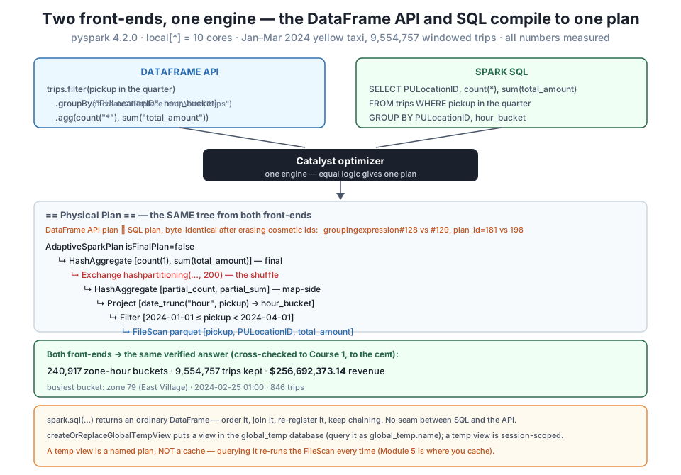
DataFrame API and Spark SQL both feed Catalyst, which compiles either into the same physical plan — byte-identical once the cosmetic node ids (#128 vs #129, plan_id=181 vs 198) are erased. Both cross-check to Course 1's ground truth exactly: 240,917 buckets, 9,554,757 trips, $256,692,373.14 revenue, busiest bucket zone 79 (East Village) at 846 trips. A temp view is a named plan, not a cache — querying it re-runs the FileScan.spark.sql(…) always returns a DataFrame
This is the mental model that unlocks free mixing. spark.sql("SELECT ...") does not return rows, a cursor, or a special result set — it returns a lazy DataFrame, exactly like spark.read.parquet(...). So you can .orderBy(...), .filter(...), .join(...), register it as another view, or hand it to a function, all without leaving the API. And the reverse holds: any DataFrame becomes SQL-addressable the moment you createOrReplaceTempView it. There is no conversion cost and no fidelity loss crossing between them, because there is nothing to convert — both are just plans headed for Catalyst.
Temporary means session-scoped, and lazy
A view registered with createOrReplaceTempView disappears when the SparkSession stops — there is no on-disk table and nothing to drop or clean up. createOrReplaceGlobalTempView widens the scope to all sessions in the application via the global_temp database (query it as global_temp.<name>), but it is still tied to the application’s lifetime, not persisted. Neither one caches: both bind a name to a plan, so each query re-executes that plan against the source files. Persisting the data is a separate, deliberate act (.cache()), which Module 5 covers.
One session all the way through, released at the end:
spark.stop()
print("session stopped")
session stoppedExercise 1 — Register, query, and confirm the return type. Read the three monthly files, register them as a temp view called rides, and write a SQL query with spark.sql(...) that returns the five busiest pickup zones over the whole quarter (group by PULocationID, count(*), order descending, limit 5). Print type(...).__name__ of what spark.sql(...) returns before you call .show(), and then, on that same result, chain a DataFrame API .withColumn(...) that adds a column — proving the SQL result is a DataFrame you can keep building on.
Hint
spark.sql(...) returns a DataFrame every time — that’s the whole point of the print. Because it’s a DataFrame, result.withColumn("note", F.lit("top zone")) works directly on it with no conversion. Your top zone should be one of the quarter’s giants from the ground truth — Midtown Center, Upper East Side South, or JFK — so if zone 237, 236, or 132 tops your list, you’re on track. If spark.sql raises TABLE_OR_VIEW_NOT_FOUND, you either forgot to call createOrReplaceTempView("rides") or misspelled the view name inside the query string.
Exercise 2 — Prove the plans match for a query you write. Pick any non-trivial query — say, average total_amount by PULocationID for trips with passenger_count > 1 — and express it both as a DataFrame API pipeline and as a SQL string over the trips view. Capture both physical plans with the plan_text/strip_ids helpers from the lesson, and assert that they are equal after erasing the cosmetic ids. Then, in one sentence, explain what the raw (un-stripped) comparison returns and why.
Hint
After strip_ids, the two plans should compare True; the raw comparison returns False because Spark stamps each query with fresh attribute ids (#123) and plan_id= node ids that increment through the session, so two logically identical plans never share the exact same numbers. If your stripped comparison comes back False, the two versions probably aren’t logically identical — check that the filter, the grouping expression, and the aggregate functions match exactly (a sum versus avg, or a > versus >=, will legitimately produce different plans).
Exercise 3 — A view is a plan, not a cache. Register the windowed report as a temp view, then run two different aggregate queries against it (for example, total revenue, then total trips). Call .explain() on each and look at the leaf node of both plans. Do they both reach a FileScan parquet, or does the second one find the data already in memory? Explain in one sentence what that tells you about whether the view stored any data.
Hint
Both plans bottom out in FileScan parquet — never an InMemoryTableScan — because a temp view stores no data at all; it stores a plan, and each query re-executes that plan from the source files. That’s why the second query re-scans instead of reusing the first query’s work. If you wanted the data held in memory so the second query skipped the scan, you’d have to call .cache() on the DataFrame and trigger an action first — the deliberate materialization step this lesson pointed toward Module 5, and explicitly distinguished from what a view does.
The DataFrame API and Spark SQL are two front-ends to one engine, and this lesson proved it rather than asserting it. Registering a DataFrame with createOrReplaceTempView("trips") makes it addressable by name inside a SQL string, and spark.sql("SELECT ...") returns an ordinary lazy DataFrame — not a special result object — which is why you can order, filter, join, or re-register it without ever leaving the API. Writing CityFlow’s zone-hour report both ways produced the identical top-five rows (zone 79, East Village, 846 trips at the peak), and under .explain() the two physical plans differed only in generated node ids: _groupingexpression#128 versus #129 and plan_id=181 versus 198. Erasing those with a regex made the plans byte-identical (True), because both were compiled by the same optimizer, Catalyst, into the same tree — an AdaptiveSparkPlan over a final HashAggregate, an Exchange, a partial HashAggregate, a Project, a Filter, and one FileScan parquet. Both routes cross-checked to Course 1’s audited ground truth to the cent: 240,917 buckets, 9,554,757 trips, $256,692,373.14 revenue. We closed on createOrReplaceGlobalTempView and the global_temp database, spark.catalog for listing views and columns, and the honest gotcha that a temp view is a named plan, not a cache — a fresh query against it shows a FileScan at the leaf, re-reading the files, because registering a view materializes nothing.
createOrReplaceTempView / spark.sql — register a DataFrame under a name, then query it as SQL; spark.sql(...) returns a lazy DataFrame, so SQL and the DataFrame API mix in one pipeline with no conversion and no seam.#N) and plan_id= node ids are erased. Neither is faster..explain() prints the physical plan; the same query shows AdaptiveSparkPlan, HashAggregate (partial then final), an Exchange shuffle, and a leaf FileScan parquet regardless of which front-end wrote it.createOrReplaceGlobalTempView / global_temp — a global view is visible to every session in the application through the global_temp database (query as global_temp.<name>); a plain temp view is session-scoped and both vanish with the application. Introspect either with spark.catalog.listTables / listColumns.FileScan, not InMemoryTableScan), so repeated querying re-scans until you deliberately .cache() in Module 5.CityFlow’s team is not monolithic: the engineers building pipelines think in composable, testable code, and the analysts answering “which zones drove revenue last quarter” think in SELECT ... GROUP BY. The fact that both dialects compile to the same Catalyst plan means those two groups are not choosing between a fast tool and a slow one, or a real API and a toy one — they are choosing the syntax that reads clearest for the work, and their results are guaranteed to agree because there is one engine underneath. That is a genuine organizational unlock: an analyst’s SQL and an engineer’s DataFrame pipeline can be trusted to produce the same $256,692,373.14 because they are the same plan. And knowing that a view is a named plan rather than stored data keeps you from a common and expensive misconception — that registering a view somehow “loads” the table — which would set you up to be surprised when a dashboard querying the same view ten times re-reads 160 MB of Parquet ten times. Seeing the FileScan at the leaf, every time, is what tells you when it’s finally worth reaching for the cache.
You just used .explain() as a lie detector — a way to prove two queries were secretly one — but you read only the shape of the plan, matching node against node. You have not yet learned to read a plan for what it tells you about the work: which node scans the files, which one shuffles data across the network, where the filter actually runs, and why the aggregate appears twice. Lesson 2, Reading .explain(), turns the plan from something you compare into something you interpret. You’ll meet .explain(mode="formatted"), "extended", and "cost", walk the four plan trees Catalyst builds — parsed, analyzed, optimized, and physical — and learn to point at any node in a real plan and say exactly what runs there and when. The FileScan, Exchange, and HashAggregate you saw flash past today become the vocabulary you’ll read fluently, and the Some(Asia/Tehran) time-zone note tucked inside that date_trunc will finally get explained. Once you can read a plan, Lesson 3 can show you Catalyst changing one — and the whole module opens up.
Keep DATATWEETS free. Help fund practical data, AI, and engineering lessons for learners worldwide.
