Title here
Summary here
Lesson 1 proved something that should reframe how you read your own code: the zone-hour report you wrote in Module 3 as a chain of DataFrame calls, and the same report written as a SQL string against a temp view, compile to a byte-identical physical plan. Both are just two ways of describing work to Catalyst, Spark’s optimizer, and Catalyst decides what actually runs. Which raises the obvious next question — the one this whole module turns on. If the engine, not your syntax, decides the work, then you need to be able to read what it decided. Otherwise you are flying an instrument you can’t see.
That instrument is .explain(), and this lesson makes you fluent in it. By the end you should be able to look at any node in a real Spark plan and say, out loud, what it does — which columns it reads, whether a filter got handed to the file format, where rows have to move between partitions, and which stage each piece of work belongs to. We’ll do it on CityFlow’s zone-hour report over the verified quarter, and we’ll do it honestly: every plan printed here is real output from a live session, paths shortened for width and nothing else. You’ll learn the four plan trees Spark builds on the way from your code to running tasks, the three ways .explain() can show you the physical one, and a repeatable method for reading a plan cold — leaves first, find the shuffles, check what got pushed. The report will land, as always, on Course 1’s ground truth to the cent: 240,917 zone-hour buckets, 9,554,757 trips kept, $256,692,373.14 revenue.
By the end of this lesson, you will be able to:
.explain() mode for the job: .explain() for the physical tree, mode="formatted" for numbered nodes with a details block (the readable default), mode="cost" for size estimates, mode="extended" for all four treesFileScan, Filter, Project, HashAggregate, Exchange — and state what it schedules, tying each Exchange back to a shuffle and a stage boundary from Module 2FileScan line, the PushedFilters, the pruned ReadSchema, and the PartitionFilters, and read the Some(Asia/Tehran) session-timezone stamp inside date_truncAdaptiveSparkPlan isFinalPlan=false as a draft and watch it become isFinalPlan=true once execution finalizes it, exposing the AQE-coalesced shuffleYou’ll need pyspark (JDK 17 or 21 — see the course setup) and the three taxi-quarter Parquet files. No new packages; .explain() is built into every DataFrame.
To learn to read plans, we need one plan worth reading — structured enough to have real parts, simple enough to hold in your head. CityFlow’s zone-hour report is exactly that: filter the quarter to the report window, group every trip by its pickup zone and its truncated pickup hour, and for each bucket count the trips and sum the revenue. It has a scan, a filter, a derived column, an aggregation, and — because a groupBy regroups rows — a shuffle. That is the anatomy of most analytical queries you will ever write.
If you’re following along on a fresh machine, fetch the quarter once from the public TLC source:
# gate: skip
# CityFlow's verified quarter, fetched once from the public TLC source.
import urllib.request
for month in ("01", "02", "03"):
    urllib.request.urlretrieve(
        f"https://d37ci6vzurychx.cloudfront.net/trip-data/yellow_tripdata_2024-{month}.parquet",
        f"yellow_tripdata_2024-{month}.parquet",
    )
Start the standard session and build the report. Notice what does not happen when you run this: nothing executes. filter, groupBy, and agg are transformations — they build a plan and return immediately (Module 2’s lazy-evaluation lesson). That is precisely why we can .explain() before spending a second of compute:
import warnings
warnings.filterwarnings("ignore")
from pyspark.sql import SparkSession
import pyspark.sql.functions as F

spark = (SparkSession.builder
         .appName("cityflow")
         .master("local[*]")
         .config("spark.ui.showConsoleProgress", "false")
         .getOrCreate())
spark.sparkContext.setLogLevel("ERROR")

QUARTER = ["yellow_tripdata_2024-01.parquet",
           "yellow_tripdata_2024-02.parquet",
           "yellow_tripdata_2024-03.parquet"]
quarter = spark.read.parquet(*QUARTER)

report = (quarter
    .filter((F.col("tpep_pickup_datetime") >= "2024-01-01") &
            (F.col("tpep_pickup_datetime") < "2024-04-01"))
    .groupBy("PULocationID",
             F.date_trunc("hour", "tpep_pickup_datetime").alias("pickup_hour"))
    .agg(F.count("*").alias("trips"),
         F.sum("total_amount").alias("revenue")))

print("report is built -- nothing has executed yet")
report is built -- nothing has executed yetreport is now a lazy DataFrame holding a plan. Everything that follows reads that plan without running it — until the very end, when we deliberately run it to see what changes.
.explain(mode="extended")When you hand Spark a query, it does not leap straight from your code to running tasks. It walks the query through four representations, each stricter and more concrete than the last, and .explain(mode="extended") prints all four so you can watch the transformation. This is the single most useful thing to run when you want to understand what Catalyst did to your query:
report.explain(mode="extended")== Parsed Logical Plan ==
'Aggregate ['PULocationID, 'date_trunc(hour, 'tpep_pickup_datetime) AS pickup_hour#20], ['PULocationID, 'date_trunc(hour, 'tpep_pickup_datetime) AS pickup_hour#20, 'count(*) AS trips#21, 'sum('total_amount) AS revenue#22]
+- Filter ((tpep_pickup_datetime#1 >= cast(2024-01-01 as timestamp_ntz)) AND (tpep_pickup_datetime#1 < cast(2024-04-01 as timestamp_ntz)))
+- Relation [VendorID#0,tpep_pickup_datetime#1,tpep_dropoff_datetime#2,passenger_count#3L,trip_distance#4,RatecodeID#5L,store_and_fwd_flag#6,PULocationID#7,DOLocationID#8,payment_type#9L,fare_amount#10,extra#11,mta_tax#12,tip_amount#13,tolls_amount#14,improvement_surcharge#15,total_amount#16,congestion_surcharge#17,Airport_fee#18] parquet
== Analyzed Logical Plan ==
PULocationID: int, pickup_hour: timestamp, trips: bigint, revenue: double
Aggregate [PULocationID#7, date_trunc(hour, cast(tpep_pickup_datetime#1 as timestamp), Some(Asia/Tehran))], [PULocationID#7, date_trunc(hour, cast(tpep_pickup_datetime#1 as timestamp), Some(Asia/Tehran)) AS pickup_hour#20, count(1) AS trips#21L, sum(total_amount#16) AS revenue#22]
+- Filter ((tpep_pickup_datetime#1 >= cast(2024-01-01 as timestamp_ntz)) AND (tpep_pickup_datetime#1 < cast(2024-04-01 as timestamp_ntz)))
+- Relation [VendorID#0,tpep_pickup_datetime#1,...,Airport_fee#18] parquet
== Optimized Logical Plan ==
Aggregate [PULocationID#7, _groupingexpression#44], [PULocationID#7, _groupingexpression#44 AS pickup_hour#20, count(1) AS trips#21L, sum(total_amount#16) AS revenue#22]
+- Project [PULocationID#7, total_amount#16, date_trunc(hour, cast(tpep_pickup_datetime#1 as timestamp), Some(Asia/Tehran)) AS _groupingexpression#44]
+- Filter (isnotnull(tpep_pickup_datetime#1) AND ((tpep_pickup_datetime#1 >= 2024-01-01 00:00:00) AND (tpep_pickup_datetime#1 < 2024-04-01 00:00:00)))
+- Relation [VendorID#0,tpep_pickup_datetime#1,...,Airport_fee#18] parquet
== Physical Plan ==
AdaptiveSparkPlan isFinalPlan=false
+- HashAggregate(keys=[PULocationID#7, _groupingexpression#44], functions=[count(1), sum(total_amount#16)], output=[PULocationID#7, pickup_hour#20, trips#21L, revenue#22])
+- Exchange hashpartitioning(PULocationID#7, _groupingexpression#44, 200), ENSURE_REQUIREMENTS, [plan_id=15]
+- HashAggregate(keys=[PULocationID#7, _groupingexpression#44], functions=[partial_count(1), partial_sum(total_amount#16)], output=[PULocationID#7, _groupingexpression#44, count#47L, sum#48])
+- Project [PULocationID#7, total_amount#16, date_trunc(hour, cast(tpep_pickup_datetime#1 as timestamp), Some(Asia/Tehran)) AS _groupingexpression#44]
+- Filter ((isnotnull(tpep_pickup_datetime#1) AND (tpep_pickup_datetime#1 >= 2024-01-01 00:00:00)) AND (tpep_pickup_datetime#1 < 2024-04-01 00:00:00))
+- FileScan parquet [tpep_pickup_datetime#1,PULocationID#7,total_amount#16] Batched: true, DataFilters: [isnotnull(tpep_pickup_datetime#1), ...], Format: Parquet, Location: InMemoryFileIndex(3 paths)[file:.../de-work/yellow_tripdata_2024-*.parquet], PartitionFilters: [], PushedFilters: [IsNotNull(tpep_pickup_datetime), GreaterThanOrEqual(tpep_pickup_datetime,2024-01-01T00:00), Less..., ReadSchema: struct<tpep_pickup_datetime:timestamp_ntz,PULocationID:int,total_amount:double>(Two long lines are shortened: the full 19-column Relation list is elided to ...,Airport_fee#18, and the FileScan absolute path is replaced with file:.../de-work/... — nothing else is changed.) Read the four trees top to bottom, and give each its job:
Parsed Logical Plan — the raw syntax tree, straight from your code. Look at the tick marks: 'PULocationID, 'count(*), 'total_amount. In Catalyst’s notation a leading apostrophe means unresolved — the parser knows you wrote the name PULocationID, but it has not yet checked that such a column exists, what type it is, or whether count(*) is a legal thing to ask of it. This tree is pure structure: an Aggregate over a Filter over a Relation, faithful to what you typed and nothing more. It is the plan at its most naive.
Analyzed Logical Plan — the same tree after Catalyst has consulted the catalog (the registry of tables, views, and columns from Lesson 1) and resolved every reference. Three things just appeared that weren’t there a moment ago. First, a schema line up top: PULocationID: int, pickup_hour: timestamp, trips: bigint, revenue: double — the analyzer now knows the output types. Second, the tick marks are gone and names carry IDs (PULocationID#7): each column is bound to a specific, existing attribute. Third — and note this, it recurs all lesson — date_trunc gained a third argument, Some(Asia/Tehran): the analyzer stamped the session timezone into the truncation, because truncating a timestamp to the hour is only well-defined against a zone. This is the stage that would have thrown an AnalysisException if you had misspelled a column; resolution is where Spark validates your query against reality.
Optimized Logical Plan — the analyzed tree after Catalyst’s rule-based optimizer has rewritten it, and this is where the engine starts earning its keep. Compare it line by line to the analyzed plan and you can see the rewrites. The Filter predicate changed: isnotnull(tpep_pickup_datetime#1) was hoisted to the front (a null check is cheap and can short-circuit the rest), and cast(2024-01-01 as timestamp_ntz) collapsed to the literal 2024-01-01 00:00:00 — constant folding, computing the cast once at plan time instead of once per row. And a brand-new Project node appeared between the filter and the aggregate, pulling out PULocationID, total_amount, and the truncated-hour expression as _groupingexpression#44 — Catalyst deciding exactly which columns flow upward, the first move of column pruning. (Lesson 3 makes these optimizations the whole subject, shown as before-and-after diffs; here, just register that the optimized tree is genuinely different from what you wrote.)
Physical Plan — the optimized logical tree turned into concrete executable operators, and the only tree that describes actual work. The logical Aggregate became a pair of HashAggregates with an Exchange between them; the logical Relation became a FileScan parquet that lists the three columns it will read and the filters it will push into the file format. This is the tree you will spend most of your plan-reading life inside, so the rest of the lesson lives here.
The takeaway of the four trees: your code is a request, not a program. Between what you wrote and what runs, Catalyst validates it, rewrites it, and compiles it — and mode="extended" is the X-ray that shows all three happening.
Most of the time you don’t want all four trees — you want the physical one, the tree that runs. Spark gives you three lenses on it, and knowing which to reach for saves real time.
The plain .explain() prints the physical tree by itself:
report.explain()== Physical Plan ==
AdaptiveSparkPlan isFinalPlan=false
+- HashAggregate(keys=[PULocationID#7, _groupingexpression#44], functions=[count(1), sum(total_amount#16)])
+- Exchange hashpartitioning(PULocationID#7, _groupingexpression#44, 200), ENSURE_REQUIREMENTS, [plan_id=15]
+- HashAggregate(keys=[PULocationID#7, _groupingexpression#44], functions=[partial_count(1), partial_sum(total_amount#16)])
+- Project [PULocationID#7, total_amount#16, date_trunc(hour, cast(tpep_pickup_datetime#1 as timestamp), Some(Asia/Tehran)) AS _groupingexpression#44]
+- Filter ((isnotnull(tpep_pickup_datetime#1) AND (tpep_pickup_datetime#1 >= 2024-01-01 00:00:00)) AND (tpep_pickup_datetime#1 < 2024-04-01 00:00:00))
+- FileScan parquet [tpep_pickup_datetime#1,PULocationID#7,total_amount#16] Batched: true, DataFilters: [isnotnull(tpep_pickup_datetime#1), ...], PushedFilters: [IsNotNull(tpep_pickup_datetime), GreaterThanOrEqual(tpep_pickup_datetime,2024-01-01T00:00), Less..., ReadSchema: struct<tpep_pickup_datetime:timestamp_ntz,PULocationID:int,total_amount:double>(The FileScan line’s Location path is dropped and its PushedFilters list is truncated by Spark itself with ....) This is compact and gives you the tree shape at a glance — but notice the frustration built into it: the PushedFilters list runs off the end with ..., and long nodes wrap into an unreadable smear. For anything beyond a glance, use the next mode.
.explain(mode="formatted") is the readable default, and the one to build the habit around. It splits the output in two: a clean tree of numbered nodes at the top, then a details block that expands each number with its inputs, outputs, and arguments — no truncation:
report.explain(mode="formatted")== Physical Plan ==
AdaptiveSparkPlan (7)
+- HashAggregate (6)
+- Exchange (5)
+- HashAggregate (4)
+- Project (3)
+- Filter (2)
+- Scan parquet (1)
(1) Scan parquet
Output [3]: [tpep_pickup_datetime#1, PULocationID#7, total_amount#16]
Batched: true
Location: InMemoryFileIndex [file:.../de-work/yellow_tripdata_2024-01.parquet, ... 2 entries]
PushedFilters: [IsNotNull(tpep_pickup_datetime), GreaterThanOrEqual(tpep_pickup_datetime,2024-01-01T00:00), LessThan(tpep_pickup_datetime,2024-04-01T00:00)]
ReadSchema: struct<tpep_pickup_datetime:timestamp_ntz,PULocationID:int,total_amount:double>
(2) Filter
Input [3]: [tpep_pickup_datetime#1, PULocationID#7, total_amount#16]
Condition : ((isnotnull(tpep_pickup_datetime#1) AND (tpep_pickup_datetime#1 >= 2024-01-01 00:00:00)) AND (tpep_pickup_datetime#1 < 2024-04-01 00:00:00))
(3) Project
Output [3]: [PULocationID#7, total_amount#16, date_trunc(hour, cast(tpep_pickup_datetime#1 as timestamp), Some(Asia/Tehran)) AS _groupingexpression#44]
Input [3]: [tpep_pickup_datetime#1, PULocationID#7, total_amount#16]
(4) HashAggregate
Input [3]: [PULocationID#7, total_amount#16, _groupingexpression#44]
Keys [2]: [PULocationID#7, _groupingexpression#44]
Functions [2]: [partial_count(1), partial_sum(total_amount#16)]
Aggregate Attributes [2]: [count#45L, sum#46]
Results [4]: [PULocationID#7, _groupingexpression#44, count#47L, sum#48]
(5) Exchange
Input [4]: [PULocationID#7, _groupingexpression#44, count#47L, sum#48]
Arguments: hashpartitioning(PULocationID#7, _groupingexpression#44, 200), ENSURE_REQUIREMENTS, [plan_id=15]
(6) HashAggregate
Input [4]: [PULocationID#7, _groupingexpression#44, count#47L, sum#48]
Keys [2]: [PULocationID#7, _groupingexpression#44]
Functions [2]: [count(1), sum(total_amount#16)]
Aggregate Attributes [2]: [count(1)#42L, sum(total_amount#16)#43]
Results [4]: [PULocationID#7, _groupingexpression#44 AS pickup_hour#20, count(1)#42L AS trips#21L, sum(total_amount#16)#43 AS revenue#22]
(7) AdaptiveSparkPlan
Output [4]: [PULocationID#7, pickup_hour#20, trips#21L, revenue#22]
Arguments: isFinalPlan=false(One Location line is path-shortened.) See how much easier this is to work with: the top tree gives you the shape and the node numbers, and the details block lets you look up node (5) and read its full hashpartitioning(..., 200) argument without it wrapping off the screen. Crucially, the PushedFilters list that got truncated above is here in full. When someone asks you “what does this plan do?”, this is the mode you screenshot.
.explain(mode="cost") adds size estimates to the optimized logical plan — Spark’s guess at how many bytes each node produces, which is what the cost-based side of the optimizer uses to make decisions like join strategy:
report.explain(mode="cost")== Optimized Logical Plan ==
Aggregate [...], Statistics(sizeInBytes=34.4 MiB)
+- Project [...], Statistics(sizeInBytes=26.8 MiB)
+- Filter (...), Statistics(sizeInBytes=153.0 MiB)
+- Relation [...] parquet, Statistics(sizeInBytes=153.0 MiB)
== Physical Plan ==
AdaptiveSparkPlan isFinalPlan=false
+- HashAggregate(keys=[PULocationID#7, _groupingexpression#44], ...)
+- Exchange hashpartitioning(PULocationID#7, _groupingexpression#44, 200), ...
... (same physical tree as above)(The node arguments are abbreviated; the Statistics(...) annotations are exact.) Read the estimates bottom-up and something important shows through. The Relation and the Filter carry the same 153.0 MiB estimate — Spark thinks the filter removes nothing, because it has no statistics about the timestamp column to estimate selectivity with. That is not a quirk; it is the honest consequence of these Parquet files shipping no column statistics, a fact that will matter enormously in Lesson 3 when we ask whether a pushed filter actually skips data. For now, notice what cost gives you and what it can’t: byte estimates, yes; accurate ones, only as good as the statistics the source provides.
Here is the skill the lesson exists to install. A physical plan is printed root-first — the AdaptiveSparkPlan at the top is the last thing that runs, and each +- indents one level deeper toward the sources. So you read it like data flows: bottom-up, leaves first. The rows are born at the FileScan and flow upward through each node to the root. Let’s walk our report’s seven nodes in the order they execute, using the formatted output’s numbers.
(1) FileScan parquet — the leaf, where every plan begins. This node reads bytes off disk and hands rows upward. Three fields on it are the ones you will read for the rest of your career:
Output [3]: [tpep_pickup_datetime#1, PULocationID#7, total_amount#16] and ReadSchema: struct<tpep_pickup_datetime, PULocationID, total_amount> — the scan reads only 3 columns, though the file has 19 (you saw all 19 in the parsed plan’s Relation). That is column pruning: Catalyst told the scan to skip the 16 columns the report never touches, and Parquet’s columnar layout means those columns are never read off disk at all.PushedFilters: [IsNotNull(...), GreaterThanOrEqual(..., 2024-01-01T00:00), LessThan(..., 2024-04-01T00:00)] — the window predicate was pushed down into the file format. Spark asks Parquet to apply the filter during the read rather than reading everything and filtering after. (An honest caveat we’ll cash out in Lesson 3: pushed does not always mean skipped — these files carry no row-group statistics, so Parquet still scans every row group and applies the predicate. Pushdown is real; the data-skipping it can enable is not, on this file.)PartitionFilters: [] — empty, because the data isn’t laid out in partition directories (like year=2024/month=01/). If it were, a filter on the partition column would appear here and prune whole directories. Worth knowing the field exists so you recognize when it’s doing work.(2) Filter — drop the out-of-window rows. Condition: isnotnull(tpep_pickup_datetime) AND (>= 2024-01-01 00:00:00) AND (< 2024-04-01 00:00:00). This looks redundant with the pushed filter below it, and partly it is — Spark applies the predicate here again as a guarantee, because pushdown is best-effort and the format may not have honored all of it. A narrow operation: it drops rows where they sit, moving nothing between partitions.
(3) Project — compute the derived column. Output shows it building _groupingexpression#44 = date_trunc(hour, cast(tpep_pickup_datetime as timestamp), Some(Asia/Tehran)). This is the truncated pickup hour becoming a real column so the aggregate can group on it. Note the Some(Asia/Tehran) again — the session timezone, riding along inside every timestamp truncation (more on that below). Also narrow; it reshapes rows in place.
(4) HashAggregate with partial_count(1), partial_sum(total_amount) — the map-side pre-aggregate. This is the first half of the groupBy, and it’s a genuinely clever move. Before moving any data, each task aggregates its own partition: it builds a hash table keyed by (zone, hour) and accumulates a partial count and partial sum per key. A task that saw a million rows but only a few thousand distinct zone-hours emits only a few thousand rows. This is why the shuffle above it stays cheap — you combine before you move.
(5) Exchange hashpartitioning(PULocationID, _groupingexpression, 200) — the shuffle. The one boundary in this plan. This is the most important node to recognize on sight. An Exchange is Spark’s plan-language for a shuffle: rows physically moving between partitions across the network. Here, hashpartitioning(..., 200) means every partial-aggregate row is routed to one of 200 target partitions by hashing its (zone, hour) key — so that every row for a given bucket lands in the same place, ready to be combined. And this ties straight back to Module 2’s DAG lesson: every Exchange is a stage boundary. Everything below this node (nodes 1–4) is one stage — the map side, scanning and pre-aggregating each partition. Everything above it (nodes 6–7) is the next stage. One Exchange, one shuffle, two stages. Counting the Exchanges in a plan is counting the shuffles is counting the stage boundaries — the same act, three vocabularies.
(6) HashAggregate with count(1), sum(total_amount) — the final aggregate. The second half of the groupBy. Now that all rows for each (zone, hour) bucket are colocated in the same partition, this node combines the partials into finished totals: it sums the partial counts into the real trip count and the partial sums into the real revenue. Its Results line renames them to your aliases — count(1) AS trips, sum(total_amount) AS revenue. This is where the 240,917 finished buckets are born.
(7) AdaptiveSparkPlan — the wrapper, not an operator. The root isn’t a step that processes rows; it’s the envelope Spark wraps every query in so that Adaptive Query Execution can re-plan the tree at runtime. Its one argument, isFinalPlan=false, is telling you something honest: this plan is a draft. Which is the next thing to understand.
The Some(Asia/Tehran) inside date_trunc
Every timestamp truncation in the plan reads date_trunc(hour, cast(...), Some(Asia/Tehran)). That Some(Asia/Tehran) is the session timezone Spark stamps into the operation, because “truncate to the hour” is only meaningful relative to a zone. It’s the machine that produced these plans reporting its local zone — set spark.sql.session.timeZone explicitly (e.g. to "UTC") if you want reproducible truncation across machines, and it will show there instead. It changes nothing about how you read the plan; just don’t be surprised to see your own zone riding inside every date_trunc and timestamp cast.
isFinalPlan=false → trueEvery physical plan we’ve printed carries AdaptiveSparkPlan isFinalPlan=false. That false is not an error — it’s Spark being honest that what you’re reading is the plan it intends to run, made from estimates, before it has seen a single real row. Adaptive Query Execution (AQE), on by default in Spark 4, executes the plan up to each shuffle, measures the real data that landed there, and re-plans everything downstream with actual numbers instead of guesses. The plan only finalizes once it has run.
So the honest way to see the final plan is to make the query execute and ask again. Accessing .rdd forces the whole thing to run:
print("partitions after AQE finalizes:", report.rdd.getNumPartitions())
report.explain()
partitions after AQE finalizes: 6
== Physical Plan ==
AdaptiveSparkPlan isFinalPlan=true
+- == Final Plan ==
ResultQueryStage 1
+- *(2) HashAggregate(keys=[PULocationID#7, _groupingexpression#44], functions=[count(1), sum(total_amount#16)])
+- AQEShuffleRead coalesced
+- ShuffleQueryStage 0
+- Exchange hashpartitioning(PULocationID#7, _groupingexpression#44, 200), ENSURE_REQUIREMENTS, [plan_id=37]
+- *(1) HashAggregate(keys=[PULocationID#7, _groupingexpression#44], functions=[partial_count(1), partial_sum(total_amount#16)])
+- *(1) Project [PULocationID#7, total_amount#16, date_trunc(hour, cast(tpep_pickup_datetime#1 as timestamp), Some(Asia/Tehran)) AS _groupingexpression#44]
+- *(1) Filter ((isnotnull(tpep_pickup_datetime#1) AND (tpep_pickup_datetime#1 >= 2024-01-01 00:00:00)) AND (tpep_pickup_datetime#1 < 2024-04-01 00:00:00))
+- *(1) ColumnarToRow
+- FileScan parquet [tpep_pickup_datetime#1,PULocationID#7,total_amount#16] ... PushedFilters: [...], ReadSchema: struct<tpep_pickup_datetime:timestamp_ntz,PULocationID:int,total_amount:double>
+- == Initial Plan ==
HashAggregate(keys=[PULocationID#7, _groupingexpression#44], functions=[count(1), sum(total_amount#16)])
+- Exchange hashpartitioning(PULocationID#7, _groupingexpression#44, 200), ENSURE_REQUIREMENTS, [plan_id=15]
+- HashAggregate(keys=[PULocationID#7, _groupingexpression#44], functions=[partial_count(1), partial_sum(total_amount#16)])
+- ... (the draft you already read)(The FileScan line is path-shortened.) Everything about the plan just got more honest, and three new things are worth naming. First, isFinalPlan=true, and the tree now splits into == Final Plan == and == Initial Plan == — AQE showing you both the draft it started with and the plan it actually ran. Second, right above the Exchange sits AQEShuffleRead coalesced, and that ties to the number printed first: the shuffle was configured for 200 partitions, but AQE looked at the real post-shuffle data — a few megabytes of partial aggregates — and decided 200 tasks was absurd overkill, coalescing them down to 6. That’s the same AQE coalescing you saw in Module 2, sized to this larger report (240,917 buckets is more than the zone leaderboard’s few hundred, so it lands on 6 partitions rather than 1). Third, the *(1) and *(2) prefixes are whole-stage code generation markers — Spark compiled each stage’s fused operators into a single generated Java method, and the numbers group nodes by stage: everything *(1) is the map stage, *(2) is the reduce stage. The boundary sits exactly at the Exchange, precisely where you predicted.
The discipline this teaches: when you .explain() a query you have not run, you are reading a forecast. It tells you the operators, the pruning, the pushdown, and where the shuffles are — all of which are decided at plan time and won’t change. What it cannot tell you is what AQE will do with runtime statistics: how the 200 will be coalesced, whether a join flips strategy. For that, run it and read isFinalPlan=true, or open the SQL tab in the Spark UI at localhost:4040, which draws the final plan after every action.
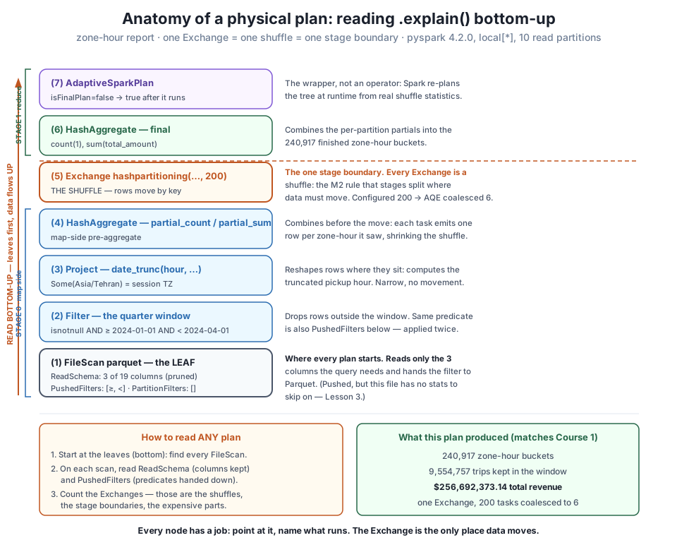
FileScan (3 of 19 columns, filters pushed) and flow up through Filter, Project, and the map-side HashAggregate (partial_count/partial_sum) into the single Exchange hashpartitioning(…, 200) — the one shuffle, the one stage boundary — then the final HashAggregate combines the partials into 240,917 buckets. AQE coalesced the configured 200 shuffle partitions to 6 at runtime (isFinalPlan flips false→true). The report matches Course 1 to the cent: 9,554,757 trips, $256,692,373.14.Reading a plan is only trustworthy if the plan computes the right answer. Run the report and hold it against Course 1’s verified ground truth:
buckets = report.count()
totals = report.agg(F.sum("trips").alias("t"),
                    F.sum("revenue").alias("r")).first()
print(f"buckets : {buckets:,}")
print(f"trips   : {totals['t']:,}")
print(f"revenue : ${totals['r']:,.2f}")
buckets : 240,917
trips : 9,554,757
revenue : $256,692,373.14Every node we named produced exactly the report Course 1 established: 240,917 zone-hour buckets, 9,554,757 trips kept inside the window (the 21 stray-stamped trips fall outside it, as always), and $256,692,373.14 in revenue — the reversals kept, no phantom dollars. The plan wasn’t just readable; it was correct. Close the session:
spark.stop()
print("session closed")
session closedAnd here is the method, distilled into something you can run on any plan you’re handed cold. (1) Print it with mode="formatted" — the numbered tree plus untruncated details. (2) Find the leaves: every FileScan, read bottom-up. On each, check ReadSchema (how many columns survived pruning) and PushedFilters (which predicates went into the format). (3) Count the Exchange nodes — those are your shuffles, your stage boundaries, and the expensive parts of the query; everything between two Exchanges is one stage. (4) For anything AQE-sensitive (coalescing, join strategy), run the query and re-read with isFinalPlan=true, or watch the SQL tab. Leaves, then Exchanges, then the runtime truth. Do it in that order every time and no plan is opaque.
Exercise 1 — Point at every node. Build a fresh, slightly different query — the per-zone daily revenue, without the hour: daily = quarter.filter((F.col("tpep_pickup_datetime") >= "2024-01-01") & (F.col("tpep_pickup_datetime") < "2024-04-01")).groupBy("PULocationID", F.to_date("tpep_pickup_datetime").alias("day")).agg(F.avg("total_amount").alias("avg_fare")). Run daily.explain(mode="formatted"), then, for each numbered node, write one sentence naming what it does and whether it’s narrow or wide. How many Exchange nodes are there, and therefore how many stages? Which node computes the average, and does it still split into a partial and a final HashAggregate?
Hint
The shape will be familiar — one groupBy means one Exchange means two stages, exactly like the report. Read the FileScan (1) node’s ReadSchema: which columns survived pruning this time? (to_date needs the timestamp; avg needs total_amount; the key needs PULocationID — so three again, but not the same three.) For the average: yes, it still splits, but look closely at the partial HashAggregate’s Functions line — an average can’t be combined by averaging partial averages, so Spark carries a partial sum and a partial count across the shuffle and divides only at the final node. That’s the same “combine before you move” trick working a little harder.
Exercise 2 — Watch the trees change. Take the report from this lesson and run report.explain(mode="extended"), but this time focus only on the difference between the analyzed and optimized logical plans. Write down every change you can spot between the two trees — there are at least four. For each, name the Catalyst optimization responsible (hint: null-check hoisting, constant folding, and the inserted Project are three of them).
Hint
Put the two trees side by side line by line. Look at the Filter condition in each: what happened to cast(2024-01-01 as timestamp_ntz) (constant folding), and what got added to the front of the AND chain (an isnotnull the analyzer’s tree didn’t have)? Then look for a node in the optimized tree that has no counterpart in the analyzed tree — the Project with _groupingexpression#44, Catalyst deciding exactly which columns to carry upward. Lesson 3 will make these diffs the whole point and measure the I/O they save; here you’re just training your eye to see that the tree you wrote and the tree that runs are not the same tree.
Exercise 3 — Draft versus final. Build a two-shuffle query so there’s more for AQE to change: ranked = report.orderBy(F.desc("revenue")). Run ranked.explain() and count the Exchange nodes and note isFinalPlan. Then force execution with ranked.rdd.getNumPartitions() and run ranked.explain() again. What does isFinalPlan say now, what AQEShuffleRead nodes appear, and how many partitions did each shuffle coalesce to? Does adding the sort change how many stages the query has?
Hint
orderBy is a wide transformation — it adds a second Exchange, this one rangepartitioning rather than hashpartitioning, so the draft plan should show two Exchanges and therefore three stages (the sort’s range-partition sampling may also add a small job, as Module 2’s final exam showed). Before running, isFinalPlan=false; after .rdd, isFinalPlan=true with the tree split into == Final Plan == and == Initial Plan ==. Look for one AQEShuffleRead coalesced per shuffle and read the coalesced counts — small, because the data crossing each boundary is tiny. The lesson to feel: the number of Exchanges was fixed at plan time (you can predict it from the code), but the coalescing was decided at runtime (you can only read it after running).
.explain() is Module 4’s instrument, and this lesson made you fluent in its output. A query walks through four representations that mode="extended" prints in order: the parsed logical plan (the raw syntax tree, columns unresolved and marked with tick apostrophes), the analyzed logical plan (every column and type resolved against the catalog, the schema line filled in, and the session timezone Some(Asia/Tehran) stamped into date_trunc), the optimized logical plan (Catalyst’s rewrites visible as diffs — isnotnull hoisted, cast literals constant-folded, a Project inserted to prune 19 columns toward 3), and the physical plan (concrete operators plus the chosen Exchange). Three modes show the physical tree: plain .explain() for a compact glance, mode="formatted" for a numbered tree with an untruncated details block — the readable default — and mode="cost" for size estimates (which revealed, honestly, that Spark can’t estimate the filter’s selectivity because the files carry no statistics). Reading the physical plan bottom-up on the zone-hour report, we named all seven nodes: FileScan parquet (3 of 19 columns via pruning, the window predicate in PushedFilters, empty PartitionFilters), Filter, Project, the map-side HashAggregate (partial_count/partial_sum), the one Exchange hashpartitioning(..., 200) that is the single shuffle and stage boundary, the final HashAggregate, and the AdaptiveSparkPlan wrapper. That wrapper reads isFinalPlan=false until the query runs; forcing execution flipped it to true, split the tree into Final and Initial plans, and exposed AQEShuffleRead coalesced shrinking the configured 200 shuffle partitions to 6. The plan computed the verified report exactly: 240,917 buckets, 9,554,757 trips, $256,692,373.14.
.explain(mode="extended") prints all four; the gap between the first and last is everything the engine did that you didn’t write.FileScan fields — ReadSchema names the columns that survived column pruning, PushedFilters names the predicates handed to the file format, and PartitionFilters names filters on directory-partition columns. Read these three on every leaf to know what I/O the query actually incurs (and remember: pushed ≠ skipped without statistics).Exchange = shuffle = stage boundary — every Exchange node is a point where rows move between partitions; counting them counts the shuffles and the stages. hashpartitioning routes by key (from groupBy/join), rangepartitioning by ordered ranges (from orderBy). These are the expensive parts of any plan.HashAggregate — a groupBy compiles to two aggregates around the shuffle: a map-side one (partial_count, partial_sum) that combines each partition before the move, and a final one that combines the partials after. It’s why the shuffle stays small.AdaptiveSparkPlan isFinalPlan — false means you’re reading a draft made from estimates; true (after the query runs) means AQE has re-planned from real runtime statistics, showing Final vs Initial plans and AQEShuffleRead coalesced where it right-sized the shuffle. Read the draft to predict; run it to know.The engineers on CityFlow’s team don’t argue about pipelines in the abstract — they paste plans. “Why is this backfill slow?” is answered by reading the .explain(mode="formatted") output: is the FileScan pruning columns or dragging all 19? Are there two Exchange nodes where there should be one? Did the filter push down, and does the data even have statistics for it to matter? Every one of those questions is now a thing you can point at in a plan and answer, which is the difference between guessing at performance and diagnosing it. The four-tree view is just as practical for correctness: when a query returns something surprising, the analyzed plan tells you whether Spark resolved your columns the way you meant, and the Some(Asia/Tehran) stamp is exactly the kind of silent assumption that turns “truncate to the hour” into an off-by-a-timezone bug across machines. And the isFinalPlan distinction keeps you honest about what a plan can promise: the operators and the shuffles are decided before you run, but the coalescing and the join strategies are decided while you run — so you read the draft to predict a query’s shape and read the final to know what it did. Predicting and reading are the two halves of controlling Spark; the next lesson gives you the third — changing it.
You’ve now seen Catalyst’s fingerprints all over the optimized plan — the hoisted isnotnull, the folded cast literals, the inserted Project that prunes columns, the PushedFilters on the scan — but only as things that appear in the output. Lesson 3, Catalyst’s Optimizations, turns each one into a controlled experiment. You’ll run the same query with and without a select, and watch ReadSchema shrink from 19 columns to 3 as a measurable I/O win. You’ll add a filter and watch PushedFilters appear — then confront the honest limit this lesson foreshadowed, because the taxi files ship no row-group statistics, so that pushed filter skips no data on them, and you’ll measure exactly that. Then you’ll build a small Parquet file that does carry statistics, and watch the same pushdown suddenly cut the input for real — the “here’s when it actually works” that makes the distinction concrete. Reading a plan told you what Spark decided; next you learn to read the diff between two plans, which is how you tell an optimization that fired from one that didn’t. Bring the vocabulary you drilled here — every optimization in Lesson 3 is a change to a node you can already name.
Keep DATATWEETS free. Help fund practical data, AI, and engineering lessons for learners worldwide.
