Title here
Summary here
Lesson 2 taught you to read a physical plan node by node: you can now point at a FileScan, a Filter, a HashAggregate, an Exchange and say what each one does. But every plan you read there arrived pre-optimized. Between the query you typed and the plan Spark ran sits Catalyst, and Catalyst had already rewritten your code before .explain() ever printed it — pruned columns you didn’t prune, pushed filters you wrote at the top down into the scan, folded arithmetic you left for later. This lesson makes that invisible rewriting visible by putting two plans side by side: the plan as you wrote it, and the plan Spark actually runs. The difference between them is Catalyst’s whole job.
CityFlow’s team is about to lean on that job. In Course 1 they hand-tuned everything: pruned columns by passing a columns= list to pyarrow, pushed filters by hand, built indexes to skip rows. Spark promises to do that automatically — and mostly it delivers. But the previous course also ended on a hard-won, uncomfortable fact about this exact dataset: the real TLC parquet ships no row-group statistics, and without statistics a pushed filter skips nothing. This lesson honours that finding instead of papering over it. You’ll watch column pruning pay for real, watch predicate pushdown appear in the plan and then measure that it skips zero rows on this file, and finally write a file where pushdown does skip — so you learn the distinction that separates people who trust the plan from people who trust the measurement: filter-pushed is not the same as data-skipped.
By the end of this lesson, you will be able to:
ReadSchema shrinking from 19 columns to 3, and 2.52x fewer bytesPushedFilters in a FileScan and then measure that on a statistics-less file it skips no row groups — separating a pushed filter from a skipped readPartitionFilters cut the scan from 2,964,624 rows to 145,240 — pushdown that actually paysYou’ll need pyspark and pyarrow. Let’s diff some plans.
Catalyst is Spark SQL’s query optimizer, and the least mystical way to describe it is also the most accurate: it is a tree of rewrite rules. Your query — whether you wrote it in the DataFrame API or as SQL — becomes a tree of logical operators (a scan at the leaves, projections and filters and aggregates stacked above). Catalyst walks that tree and applies rules, each of which pattern-matches a shape and rewrites it into a cheaper equivalent: “a filter sitting above a projection can move below it,” “a column no reader consumes can be dropped from the scan,” “1 = 1 is just true, delete it.” Most of these are rule-based (always-correct rewrites applied unconditionally); a few are cost-based (Catalyst estimates sizes and picks, like choosing a broadcast join for a small table, which Module 3 already saw it do). The pipeline runs in fixed stages — parsed → analyzed → optimized → physical — and the two that matter today are the middle pair: the analyzed plan is your query with names and types resolved but not yet rewritten, and the optimized plan is what Catalyst turned it into. You see the optimizer’s work by diffing those two. Let’s start the session and set up the diff.
import warnings
warnings.filterwarnings("ignore")
import os, time, shutil, subprocess, statistics
from pyspark.sql import SparkSession
from pyspark.sql import functions as F

spark = (SparkSession.builder
         .appName("cityflow")
         .master("local[*]")
         .config("spark.ui.showConsoleProgress", "false")
         .getOrCreate())
spark.sparkContext.setLogLevel("ERROR")

JAN = "yellow_tripdata_2024-01.parquet"
REPORT_COLS = ["tpep_pickup_datetime", "PULocationID", "total_amount"]

all_cols = spark.read.parquet(JAN).columns
print(f"the file ships {len(all_cols)} columns; the zone-hour report needs {len(REPORT_COLS)}")
print("all columns:", all_cols)
the file ships 19 columns; the zone-hour report needs 3all columns: ['VendorID', 'tpep_pickup_datetime', 'tpep_dropoff_datetime', 'passenger_count', 'trip_distance', 'RatecodeID', 'store_and_fwd_flag', 'PULocationID', 'DOLocationID', 'payment_type', 'fare_amount', 'extra', 'mta_tax', 'tip_amount', 'tolls_amount', 'improvement_surcharge', 'total_amount', 'congestion_surcharge', 'Airport_fee']Nineteen columns on disk, three the report actually reads. That gap is where the first optimization lives, and it is the one that pays without any argument.
The zone-hour report needs exactly three columns: tpep_pickup_datetime, PULocationID, total_amount. The other sixteen — vendor, distances, every fare component, the store-and-forward flag — are dead weight to this query. In Course 1 you saved that weight by hand, passing columns= to the parquet reader. Column pruning is Catalyst doing it for you: even if your code reads the whole file and then selects three columns, the optimizer pushes that projection down into the scan so the reader never touches the other sixteen on disk.
The proof is in the FileScan’s ReadSchema. Write the deliberately wasteful version — read everything, select three — and read the physical plan.
pruned = spark.read.parquet(JAN).select(*REPORT_COLS)
pruned.explain()
== Physical Plan ==
*(1) ColumnarToRow
+- FileScan parquet [tpep_pickup_datetime#20,PULocationID#26,total_amount#35] Batched: true, DataFilters: [], Format: Parquet, Location: InMemoryFileIndex(1 paths)[file:.../yellow_tripdata_2024-01.parquet], PartitionFilters: [], PushedFilters: [], ReadSchema: struct<tpep_pickup_datetime:timestamp_ntz,PULocationID:int,total_amount:double>Read the ReadSchema at the end of the FileScan line: struct<tpep_pickup_datetime:timestamp_ntz,PULocationID:int,total_amount:double> — three columns. We called spark.read.parquet(JAN) with no column list, which asks for all nineteen, and Catalyst still narrowed the scan to three because nothing downstream consumes the rest. The scan node’s column list at the front ([tpep_pickup_datetime#20,PULocationID#26,total_amount#35]) says the same thing: the leaf reads three columns, not nineteen. You wrote wasteful code and got the careful version for free.
Now measure what that saves. Two honest numbers, because they answer different questions. First, bytes off disk — the I/O the reader avoids — which we can read directly from the parquet file’s own metadata: every column chunk records its compressed size, so we sum the three report columns against all nineteen.
import pyarrow.parquet as pq

md = pq.ParquetFile(JAN).metadata
bytes_by_col = {}
for rg in range(md.num_row_groups):
    for c in range(md.num_columns):
        col = md.row_group(rg).column(c)
        bytes_by_col[col.path_in_schema] = bytes_by_col.get(col.path_in_schema, 0) + col.total_compressed_size

all_bytes = sum(bytes_by_col.values())
report_bytes = sum(bytes_by_col[c] for c in REPORT_COLS)
print(f"all 19 columns : {all_bytes:>12,} compressed bytes on disk")
print(f"3 report cols  : {report_bytes:>12,} compressed bytes  ({report_bytes/all_bytes*100:.1f}% of the file)")
print(f"pruning reads  : {all_bytes/report_bytes:.2f}x fewer bytes")
for c in REPORT_COLS:
    print(f"   {c:<24}{bytes_by_col[c]:>12,} B")
all 19 columns : 49,951,108 compressed bytes on disk
3 report cols : 19,810,094 compressed bytes (39.7% of the file)
pruning reads : 2.52x fewer bytes
tpep_pickup_datetime 12,795,757 B
PULocationID 2,103,429 B
total_amount 4,910,908 B2.52x fewer bytes, read straight from the file’s metadata — the scan touches 19,810,094 bytes instead of 49,951,108. Notice the honesty in the per-column breakdown: the three columns the report happens to need include tpep_pickup_datetime, which alone compresses to 12.8 MB because timestamps are high-entropy and resist compression. So pruning three of nineteen columns is not a 6.3x win here; it is 2.52x, because we kept one of the heaviest columns in the file. Column pruning saves exactly the bytes of the columns you drop — no more, no less — and the win depends on which columns those are.
Now the second number: wall time. We time it with the noop writer, which runs the whole query and throws the output away — it forces the scan to actually read and decode the columns without collecting anything to the driver. (You cannot measure pruning with .count(): Catalyst prunes every column for a count, since counting rows needs no column data, so both versions would read zero columns and the test would be meaningless.)
def warm_noop(dframe, reps=3):
    """Median wall time of a full scan+decode: run the query, discard the output."""
    dframe.write.format("noop").mode("overwrite").save()          # warm-up (JIT, page cache)
    times = []
    for _ in range(reps):
        t0 = time.perf_counter()
        dframe.write.format("noop").mode("overwrite").save()
        times.append(time.perf_counter() - t0)
    return statistics.median(times)

full = spark.read.parquet(JAN)                 # all 19 columns -- the select("*") case
t_full = warm_noop(full)
t_pruned = warm_noop(pruned)
print(f"scan all 19 columns : {t_full*1000:6.0f} ms")
print(f"scan 3 pruned cols  : {t_pruned*1000:6.0f} ms")
print(f"pruning is {t_full/t_pruned:.1f}x faster warm")
scan all 19 columns : 392 ms
scan 3 pruned cols : 69 ms
pruning is 5.7x faster warmSeveral times faster in wall time (5.7x on the run above), against a steady 2.52x in bytes — and the fact that the time multiple exceeds the byte multiple is itself the lesson. Reading is only half a scan’s job; the other half is decoding each column from its compressed, encoded on-disk form into in-memory batches, and that CPU cost scales with the number of columns, not just their bytes. Sixteen columns you never decode is sixteen columns’ worth of decompression and materialization skipped on top of the I/O, so the time saved runs ahead of the bytes saved on every re-run. This is why column pruning is the optimization nobody argues about: it is automatic, it is correct, and on real workloads with dozens of columns and one narrow report, it is often the single biggest thing Catalyst does for you. (The 2.52x byte ratio is exact and reproducible; the wall-time multiple drifts with machine load — the point is that it stays comfortably above the byte ratio, not its exact value.)
The second famous optimization is predicate pushdown: push a WHERE filter down into the scan so the reader can skip data that can’t match, instead of reading everything and filtering afterward. CityFlow’s dashboard asks about one zone constantly — JFK Airport, PULocationID = 132, the busiest pickup zone in January. Filter on it and read the plan.
one_zone = spark.read.parquet(JAN).select(*REPORT_COLS).where(F.col("PULocationID") == 132)
one_zone.explain()
== Physical Plan ==
*(1) Filter (isnotnull(PULocationID#46) AND (PULocationID#46 = 132))
+- *(1) ColumnarToRow
+- FileScan parquet [tpep_pickup_datetime#40,PULocationID#46,total_amount#55] Batched: true, DataFilters: [isnotnull(PULocationID#46), (PULocationID#46 = 132)], Format: Parquet, Location: InMemoryFileIndex(1 paths)[...], PartitionFilters: [], PushedFilters: [IsNotNull(PULocationID), EqualTo(PULocationID,132)], ReadSchema: struct<...>There it is: PushedFilters: [IsNotNull(PULocationID), EqualTo(PULocationID,132)]. Catalyst even inferred IsNotNull for you (a null can’t equal 132, so it’s safe and cheap to check early). The filter has been handed to the parquet reader. The reputation says the rest writes itself: the reader consults each row group’s min/max statistics, sees which ones can’t contain 132, and skips them.
Except this is the file Course 1’s indexing lesson opened the footer on and found empty. Let’s not take the plan’s word for it — let’s check the file, exactly as that lesson taught: an index is a property of the file, not the format.
pu_idx = [md.schema.column(i).name for i in range(md.num_columns)].index("PULocationID")
print("PULocationID row-group statistics in the real TLC file:")
for i in range(md.num_row_groups):
    col = md.row_group(i).column(pu_idx)
    print(f"   rg{i}: rows={md.row_group(i).num_rows:>9,}  is_stats_set={col.is_stats_set}  statistics={col.statistics}")
PULocationID row-group statistics in the real TLC file:
rg0: rows=1,048,576 is_stats_set=False statistics=None
rg1: rows=1,048,576 is_stats_set=False statistics=None
rg2: rows= 867,472 is_stats_set=False statistics=NoneNo statistics, on any row group. is_stats_set = False, statistics = None — the same finding Course 1 recorded, verified again here on the same file. There is no min/max for the pushed filter to compare against. The reader was handed EqualTo(PULocationID, 132) and has nothing to test it against at the row-group level, so it cannot rule out a single one of the three row groups. It must read all of them and apply the predicate row by row.
So does the pushed filter save any I/O? Measure it. If pushdown were skipping data, the filtered scan would read fewer bytes and finish faster than the unfiltered one. Time both.
t_filtered = warm_noop(one_zone)
t_unfiltered = warm_noop(pruned)   # same 3 columns, no filter
matched = one_zone.count()
print(f"scan + push filter PU=132 : {t_filtered*1000:6.0f} ms")
print(f"scan, no filter           : {t_unfiltered*1000:6.0f} ms")
print(f"rows the scan must read   : {full.count():>12,}  (all 3 row groups -- nothing skipped)")
print(f"rows the filter keeps     : {matched:>12,}  (JFK, applied AFTER the scan)")
scan + push filter PU=132 : 55 ms
scan, no filter : 62 ms
rows the scan must read : 2,964,624 (all 3 row groups -- nothing skipped)
rows the filter keeps : 145,240 (JFK, applied AFTER the scan)The two times are the same — within noise, and if anything the filtered version is a hair faster only because applying a cheap integer predicate lets a few batches shrink before the discard. The scan read all 2,964,624 rows either way. The filter is real and it is doing real work — it narrows the result to 145,240 JFK trips (which cross-checks the ground truth exactly: Course 1 pinned January’s busiest zone at JFK with 145,240 trips) — but it does that work downstream of the scan, on rows already read, not by skipping reads. This is the distinction to carve into memory:
A pushed filter is not a skipped read.
PushedFiltersin the plan means Catalyst offered the predicate to the reader. Whether the reader can skip anything with it depends on statistics the file may or may not carry — and this file carries none.
Believing PushedFilters implies data-skipping is the single most common misreading of a Spark plan. The plan tells you the optimizer’s intent; only the file’s metadata tells you the payoff.
Read the plan, then read the footer
PushedFilters: [...] is necessary but not sufficient for a skip. Before you promise anyone that a filter makes a query cheap, open the file: pq.ParquetFile(path).metadata.row_group(0).column(j).statistics. If it prints None, the filter will be evaluated on every row of every row group, no matter how confident the plan looks. The plan is a statement about the query; the footer is a statement about the file, and only the second one decides whether bytes get skipped.
The honest counter-demonstration: make a file where the skip is real, so the contrast is undeniable. The TLC file can’t skip because it lacks the metadata; the fix is to write our own copy with structure the reader can prune against. The bluntest, most reliable form of that structure is partitioning — df.write.partitionBy("PULocationID") writes one directory per zone, and the value lives in the directory name rather than inside the data. A filter on a partition column then becomes a directory decision the reader makes before opening any file: no statistics required, no rows read to find out.
PART = "c2m4l3_trips_partitioned.parquet"
if os.path.exists(PART):
    shutil.rmtree(PART)

t0 = time.perf_counter()
pruned.write.partitionBy("PULocationID").mode("overwrite").parquet(PART)
write_secs = time.perf_counter() - t0

part_dirs = [d for d in os.listdir(PART) if d.startswith("PULocationID=")]
print(f"wrote {PART} in {write_secs:.1f}s")
print(f"partition directories: {len(part_dirs)}  (one per zone that appears in the month)")
print("examples:", sorted(part_dirs)[:4], "...")
wrote c2m4l3_trips_partitioned.parquet in 5.5s
partition directories: 260 (one per zone that appears in the month)
examples: ['PULocationID=1', 'PULocationID=10', 'PULocationID=100', 'PULocationID=101'] ...Two hundred and sixty directories, one per zone. Now read the plan for the same JFK filter against this partitioned file.
part_zone = spark.read.parquet(PART).where(F.col("PULocationID") == 132)
part_zone.explain()
== Physical Plan ==
*(1) ColumnarToRow
+- FileScan parquet [tpep_pickup_datetime#66,total_amount#67,PULocationID#68] Batched: true, DataFilters: [], Format: Parquet, Location: InMemoryFileIndex(1 paths)[.../PULocationID=132], PartitionFilters: [isnotnull(PULocationID#68), (PULocationID#68 = 132)], PushedFilters: [], ReadSchema: struct<tpep_pickup_datetime:timestamp_ntz,total_amount:double>The filter has moved. On the TLC file it was a PushedFilters (offered to the reader, skipped nothing); here it is a PartitionFilters: [isnotnull(PULocationID#68), (PULocationID#68 = 132)], and PushedFilters is now empty. Look at the Location too: InMemoryFileIndex(1 paths)[.../PULocationID=132] — one path, not 260. Spark resolved the filter to a single directory at planning time and will open only that one. Measure the skip three ways: bytes on disk, rows the scan touches, and wall time.
def dir_bytes(path):
    return int(subprocess.run(["du", "-sk", path], capture_output=True, text=True).stdout.split()[0]) * 1024

whole = dir_bytes(PART)
just_132 = dir_bytes(os.path.join(PART, "PULocationID=132"))
rows_132 = spark.read.parquet(os.path.join(PART, "PULocationID=132")).count()
rows_all = spark.read.parquet(PART).count()

t_part_filter = warm_noop(part_zone)
t_part_full = warm_noop(spark.read.parquet(PART).select(*REPORT_COLS))

print(f"{'':24}{'partitioned + filter':>22}{'partitioned, full':>20}")
print(f"{'bytes read from disk':24}{just_132:>22,}{whole:>20,}")
print(f"{'rows the scan touches':24}{rows_132:>22,}{rows_all:>20,}")
print(f"{'warm wall time (ms)':24}{t_part_filter*1000:>22.0f}{t_part_full*1000:>20.0f}")
print(f"\npartition pruning reads {whole/just_132:.1f}x fewer bytes and {rows_all/rows_132:.1f}x fewer rows")
partitioned + filter partitioned, full
bytes read from disk 1,216,512 30,195,712
rows the scan touches 145,240 2,964,624
warm wall time (ms) 47 163
partition pruning reads 24.8x fewer bytes and 20.4x fewer rowsNow pushdown pays. The scan reads 1,216,512 bytes instead of 30,195,712 (24.8x fewer) and touches 145,240 rows instead of 2,964,624 (20.4x fewer), because 259 of the 260 directories were eliminated before a single file was opened — and the wall time falls sharply with it. Put the two filter demos side by side and the whole lesson is in the diff: the same PULocationID = 132 predicate skipped nothing on the real TLC file (no statistics to prune against) and skipped 95% on the partitioned file (the value is in the path). The predicate never changed. What changed is whether the file’s physical layout let the reader act on it — the exact conclusion Course 1 reached about sorting and row-group statistics, arriving here through partitioning instead.
And notice the row count that survives is 145,240 in both demos — the same JFK answer. Skipping changes the work, never the answer. That is the invariant every optimization in this lesson preserves.
Partitioning is a tool with a cost, not a free win
Partitioning made the skip real, but it isn’t free and it isn’t always right. Writing 260 directories took several seconds, and partitioning by a high-cardinality column (imagine one directory per second of pickup time) produces a swarm of tiny files that wrecks read performance — the “small files problem” Module 5 tackles. Partition by a column you filter on often and whose cardinality is modest (a few hundred zones, a handful of dates), and let row-group statistics — when the writer actually emits them — handle the finer-grained columns. The judgment, not the mechanism, is the skill.
The big two optimizations are I/O rewrites. Catalyst runs dozens of smaller ones too, and the cleanest way to catch them is to diff the analyzed plan (your query, resolved but not rewritten) against the optimized plan (Catalyst’s version). Two quick ones.
Constant folding evaluates constant expressions once, at planning time, instead of per row. Write a filter with an obviously constant term — WHERE 1 = 1 AND total_amount > 5 — and diff the plans.
folded = spark.read.parquet(JAN).select("PULocationID", "total_amount").where((F.lit(1) == F.lit(1)) & (F.col("total_amount") > 5))
print("--- ANALYZED (as written) ---")
print(folded._jdf.queryExecution().analyzed().toString().split("\n")[0])
print("--- OPTIMIZED (Catalyst) ---")
print(folded._jdf.queryExecution().optimizedPlan().toString().split("\n")[1])
--- ANALYZED (as written) ---
Filter ((1 = 1) AND (total_amount#16 > cast(5 as double)))
--- OPTIMIZED (Catalyst) ---
+- Filter (isnotnull(total_amount#16) AND (total_amount#16 > 5.0))The analyzed filter carries (1 = 1) verbatim and a runtime cast(5 as double). The optimized filter has folded both: (1 = 1) is gone entirely (it’s always true, so it contributes nothing and Catalyst deletes it), and cast(5 as double) became the literal 5.0, computed once instead of 2,964,624 times. Catalyst also slipped in isnotnull(total_amount) — the same free inference it made for the JFK filter. Three rewrites, one line, and you’d never write 1 = 1 on purpose — but real queries accumulate exactly this kind of dead constant through templating, generated SQL, and defensive AND clauses, and Catalyst sweeps them.
Filter reordering (pushing a filter past a projection) moves a WHERE as close to the scan as it can go, so fewer rows flow through the more expensive operators above it. Build the report column and then filter, so the filter sits above the projection as written.
reordered = (spark.read.parquet(JAN)
             .withColumn("hour", F.date_trunc("hour", "tpep_pickup_datetime"))
             .select("hour", "PULocationID", "total_amount")
             .where(F.col("PULocationID") == 132))
print("--- ANALYZED: filter sits ABOVE the projection ---")
for line in reordered._jdf.queryExecution().analyzed().toString().split("\n")[:2]:
    print(line)
print("--- OPTIMIZED: filter pushed BELOW it, next to the scan ---")
for line in reordered._jdf.queryExecution().optimizedPlan().toString().split("\n")[:2]:
    print(line)
--- ANALYZED: filter sits ABOVE the projection ---
Filter (PULocationID#119 = 132)
+- Project [hour#132, PULocationID#119, total_amount#128]
--- OPTIMIZED: filter pushed BELOW it, next to the scan ---
Project [date_trunc(hour, cast(tpep_pickup_datetime#113 as timestamp), Some(Asia/Tehran)) AS hour#132, PULocationID#119, total_amount#128]
+- Filter (isnotnull(PULocationID#119) AND (PULocationID#119 = 132))As written, the Filter is the top node and the Project (which computes hour via date_trunc) is below it — meaning the plan would compute hour for all 2,964,624 rows and then throw away the 95% that aren’t JFK. Catalyst flipped them: in the optimized plan the Filter is now below the Project, so the expensive date_trunc runs only on the 145,240 rows that survive the filter. (The Some(Asia/Tehran) inside date_trunc is the session time zone printing in the plan, exactly as Lesson 2 noted — harmless, and worth recognizing so it doesn’t distract you.) You wrote “compute, then filter”; Catalyst runs “filter, then compute,” because a filter that commutes past a projection always should move down. Same answer, less work above the scan.
Four rewrites, one instrument. You never told Spark to prune columns, push a filter, fold a constant, or reorder a projection — you wrote plain queries and diffed the plans to watch Catalyst do all four. The figure collects the real numbers: the genuine 2.52x byte win of pruning, the honest zero-skip of pushdown on a stats-less file, and the 20.4x skip once you give the reader a layout it can prune.
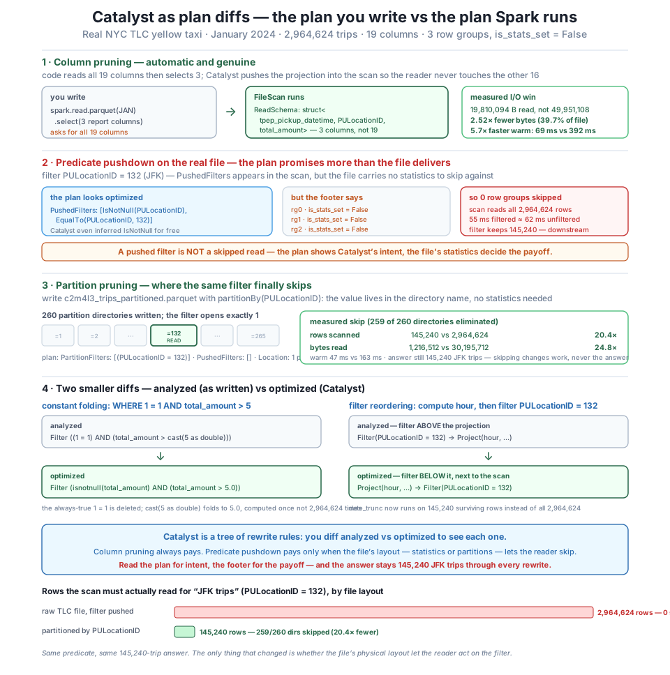
ReadSchema shrinks 19→3, scanning 19,810,094 B instead of 49,951,108 (2.52× fewer bytes, ~5.7× faster warm). Predicate pushdown is honest about its limit: PushedFilters appears for PULocationID = 132, but the file's row groups are all is_stats_set = False, so zero are skipped — the scan reads all 2,964,624 rows and the filter only narrows to 145,240 afterward. Partition pruning makes the skip real: written partitionBy(PULocationID), the same filter becomes a PartitionFilters that opens 1 of 260 directories — 145,240 rows and 1,216,512 B instead of 2,964,624 and 30,195,712 (20.4× / 24.8×). Constant folding erases 1 = 1; filter reordering slides a filter below a projection. A pushed filter is not a skipped read — the plan shows intent, the file's metadata decides the payoff, and the answer is 145,240 either way.Clean up the parquet we wrote, and close the session.
shutil.rmtree(PART)
print(f"removed {PART}")
spark.stop()
removed c2m4l3_trips_partitioned.parquetExercise 1 — Prune to the bone and measure the biggest possible win. The lesson’s three report columns included the heavy tpep_pickup_datetime, so pruning saved only 2.52x of the bytes. Pick the three smallest columns instead: use the bytes_by_col dictionary to find them, select just those three, and compute the byte ratio against all nineteen and against the report columns. Then read the physical plan and confirm ReadSchema lists your three. Explain in a comment why the byte win for the smallest columns is far larger than 2.52x even though it is still “3 of 19 columns.”
Hint
sorted(bytes_by_col.items(), key=lambda kv: kv[1])[:3] gives the three cheapest columns. You’ll find they sum to a tiny fraction of the file, so pruning to them reads maybe 20–30x fewer bytes, not 2.52x. The count of columns dropped tells you almost nothing about the bytes saved; column pruning’s payoff is measured in bytes, and bytes are wildly unequal — one high-entropy timestamp column can outweigh a dozen small integer ones. This is the same “count the bytes, not the columns” discipline Course 1 applied to dtypes.
Exercise 2 — Give the reader statistics and watch pushdown wake up (partially). The TLC file skipped nothing because it has no row-group statistics. Write your own copy of the three report columns unsorted but with statistics on — pruned.write.mode("overwrite").parquet("c2m4l3_stats.parquet") (pyarrow-written Spark parquet emits statistics by default) — then open its footer with pq.ParquetFile(...).metadata and print the PULocationID min/max per row group. Filter on PULocationID == 132, read the plan, and reason about how many row groups could be skipped. Remove the file when done. Explain why statistics help less than the partitioning demo did.
Hint
You’ll see real min/max ranges this time instead of None — but because the data isn’t sorted by PULocationID, most row groups will span a wide range of zone IDs that includes 132, so few or none can be excluded. This is exactly Course 1’s finding transplanted to a different column: statistics make bounds correct, but only clustering (sorting or partitioning by the filtered column) makes them tight enough to skip. Partitioning won so decisively because it is clustering taken to its extreme — one value per directory. Don’t forget shutil.rmtree or os.remove on the file, and keep the c2m4l3_ prefix.
Exercise 3 — Catch a filter that can’t be pushed. Column pruning and constant folding are unconditional, but filter pushdown only fires for predicates the reader understands. Build two filters on the January file: one on total_amount > 5 (a simple column comparison) and one on a computed column, F.date_trunc("hour", "tpep_pickup_datetime") == "2024-01-15 08:00:00". Read both physical plans and compare their PushedFilters lists. Explain in a comment which predicate reached the scan and which stayed in a Filter node above it, and why an expression Catalyst can’t translate to the parquet reader’s vocabulary can never be pushed — a limitation that becomes the whole story of the next lesson.
Hint
total_amount > 5 shows up in PushedFilters as GreaterThan(total_amount,5.0); the date_trunc predicate does not — it stays as a Filter node above the scan, because the parquet reader has no notion of date_trunc and Catalyst only pushes predicates it can express in the reader’s small filter vocabulary (equalities, comparisons, IsNotNull, In). The moment a filter wraps the column in a function the reader can’t evaluate, pushdown stops at the plan boundary. That boundary — expressions the optimizer can’t see through — is exactly what a Python UDF makes permanent, which is Lesson 4’s subject.
You made Catalyst visible by diffing the plan you wrote against the plan Spark ran. Column pruning is the automatic, uncontested win: spark.read.parquet(JAN).select(*REPORT_COLS) reads all nineteen columns in your code but the FileScan’s ReadSchema shrank to the three the report uses, cutting scanned bytes from 49,951,108 to 19,810,094 (a steady 2.52x) and warm wall time by several times more than that — the time win beating the byte win because sixteen columns are never decoded, not just never read. Predicate pushdown was the honest one: filtering on PULocationID == 132 made PushedFilters: [IsNotNull(PULocationID), EqualTo(PULocationID,132)] appear in the scan, but every row group of the real TLC file reports is_stats_set = False, so zero row groups were skipped — the scan read all 2,964,624 rows whether filtered or not (55 ms vs 62 ms, identical within noise), and the filter only narrowed the result to 145,240 JFK trips downstream. filter-pushed is not data-skipped. To see a real skip you wrote c2m4l3_trips_partitioned.parquet partitioned by PULocationID into 260 directories; the same filter became a PartitionFilters opening 1 directory of 260, reading 145,240 rows and 1,216,512 bytes instead of 2,964,624 and 30,195,712 — a 20.4x row cut and 24.8x byte cut, for a one-time write of a few seconds. Two smaller diffs closed it out: constant folding deleted 1 = 1 and turned cast(5 as double) into 5.0, and filter reordering slid a filter below a projection so date_trunc ran on 145,240 rows instead of 2,964,624. Every rewrite changed the work; none changed the answer, which stayed 145,240 throughout.
*. Its payoff is the summed bytes of the dropped columns (here 2.52x, because one kept timestamp column is heavy), and its time win exceeds its byte win because skipped columns are also never decoded.PushedFilters in the plan is Catalyst offering the predicate to the reader; whether the reader skips anything depends on file statistics. On the stats-less TLC file (is_stats_set = False), the pushed PULocationID filter skipped zero of 2,964,624 rows and only narrowed the result afterward. Read the footer, not just the plan.PULocationID = 132 predicate skipped nothing on the raw file and 95% on a partitionBy(PULocationID) copy, because the partition value lives in the directory path and needs no statistics. Partitioning is clustering taken to its extreme: one value per directory, pruned before a file is opened — at the cost of the write and the small-files risk of high cardinality.1 = 1, filter reordering moved date_trunc above 145,240 rows instead of below 2,964,624, and every demo returned the same 145,240 JFK trips. That invariant is what lets you trust an optimizer you can’t see: it is allowed to make the plan cheaper only in ways that are provably equivalent.CityFlow’s team was about to rewrite Course 1’s hand-tuned pipeline and trust Spark to do the pruning and pushing for them — and this lesson says they can trust column pruning completely and must verify predicate pushdown every time. A teammate who reads PushedFilters in a plan and reports “the filter is pushed, the query is optimized” is telling the truth about the plan and possibly nonsense about the file: on this exact dataset that pushed filter reads 100% of the data, forever, and nothing in the plan warns them. The engineer who instead opens the footer, sees is_stats_set = False, and either partitions the write or sorts and re-emits with statistics is the one whose dashboard query actually skips data. That is the difference between reading a plan and understanding a system: the plan states Catalyst’s intent, the file’s physical layout decides the payoff, and only measuring both tells you which query you really shipped. You can now predict and read what Spark’s optimizer does — and catch it, honestly, where the file won’t let it deliver.
Every optimization in this lesson worked by Catalyst seeing through your query — reading which columns you consume, which predicates commute past which projections, which constants are dead. Lesson 4, UDFs and Their Cost, is what happens when you hand Catalyst something it cannot see through. A Python UDF is an opaque box to the optimizer: it can’t prune columns the UDF might read, can’t push a filter phrased inside it, can’t fold or reorder around it, and every row must leave the JVM, cross into a Python process, and come back. You’ll measure the same computation four ways — a built-in F.* expression, a plain Python udf, a vectorized pandas_udf, and a SQL expression — and watch the opaque BatchEvalPython node appear in the plan exactly where pushdown and pruning stop. Exercise 3’s un-pushable date_trunc filter was the gentle version of this boundary; the UDF makes it a wall, and the lesson measures precisely what that wall costs.
Keep DATATWEETS free. Help fund practical data, AI, and engineering lessons for learners worldwide.
