Title here
Summary here
The last three lessons all rested on a single fact: Catalyst can optimize your query because it understands it. It knows filter(col("trip_distance") >= 10) is a comparison, so it can push that comparison into the file scan; it knows select drops columns, so it can prune them; it knows groupBy(...).sum(...) is an aggregation, so it can pre-aggregate on each partition before the shuffle. Every optimization you have watched depends on the engine being able to see inside the operation. This lesson is about the operation Catalyst cannot see inside: a user-defined function, a chunk of your own Python that the optimizer must treat as a black box — feed it rows, take back results, and understand nothing about what happened in between.
That opacity has a price, and the price is measurable. You’ll take one honest task — sorting January’s 2,964,624 trips into distance tiers — and express it three ways: a built-in F.when expression, the same logic as a SQL CASE, and a Python UDF. The built-in and SQL versions will finish in about a tenth of a second because they compile into the JVM and fuse into whole-stage codegen; the UDF will take seven times longer, because every one of the three million values has to cross out of the JVM into a Python process, get classified, and cross back. You’ll see the difference in the plan — a fused Project versus an opaque BatchEvalPython node — and watch a filter push cleanly into the scan for the built-in but stall helplessly above the UDF. By the end you’ll understand exactly why the rule “prefer built-in functions” is not style advice but a performance decision with a number attached.
By the end of this lesson, you will be able to:
BatchEvalPython node in a physical plan and recognize what it meansF.* first, vectorized UDFs when you must go to Python, plain Python UDFs lastYou’ll need pyspark with its Java runtime. Let’s measure the boundary of the optimizer.
The task is a distance tiering: label every trip long (10 miles or more), medium (2 to 10), or short (under 2). It is deliberately simple, because the point is not the logic but how you express it to Spark. We’ll cache one month so every measurement hits the same in-memory data rather than re-reading the file.
There is one configuration line here that matters, and it is honest about the environment. Spark 4 can run Python UDFs through Apache Arrow for speed, and it offers pandas_udf for vectorized Python — but that Arrow path is fragile against the installed pandas version, and on some pandas 3.x builds it deadlocks outright. So we pin the classic, always-correct UDF execution path explicitly. (More on the vectorized alternative, and this exact compatibility trap, at the end.)
import warnings; warnings.filterwarnings("ignore")
import time
from pyspark.sql import SparkSession, functions as F
from pyspark.sql.types import StringType

spark = (SparkSession.builder
         .appName("cityflow-udf")
         .master("local[*]")
         .config("spark.ui.showConsoleProgress", "false")
         .config("spark.sql.execution.pythonUDF.arrow.enabled", "false")
         .getOrCreate())
spark.sparkContext.setLogLevel("ERROR")

jan = spark.read.parquet("yellow_tripdata_2024-01.parquet").select("trip_distance", "total_amount")
jan.cache()
print("rows cached:", f"{jan.count():,}")
rows cached: 2,964,624Now the three expressions. The built-in uses F.when(...).otherwise(...), a native Catalyst expression. The SQL is the identical logic as a CASE statement over a temp view (Lesson 1 proved these compile to the same engine). The UDF wraps a plain Python function with F.udf, telling Spark its return type is a string:
# 1) built-in expression — native Catalyst, runs in the JVM
tier_builtin = (F.when(F.col("trip_distance") >= 10, "long")
                 .when(F.col("trip_distance") >= 2, "medium")
                 .otherwise("short"))

# 2) SQL CASE — same engine, different syntax (Lesson 1)
jan.createOrReplaceTempView("trips")
sql_query = ("SELECT CASE WHEN trip_distance >= 10 THEN 'long' "
             "WHEN trip_distance >= 2 THEN 'medium' ELSE 'short' END AS tier, "
             "COUNT(*) AS n FROM trips GROUP BY 1")

# 3) Python UDF — your code, opaque to the optimizer
def tier_py(d):
    if d is None:
        return "short"
    return "long" if d >= 10 else ("medium" if d >= 2 else "short")

tier_udf = F.udf(tier_py, StringType())
Before timing anything, confirm all three agree — a fast wrong answer is worthless, and this is the cross-check the whole course insists on:
def tier_counts(df, col):
    rows = df.groupBy(col).agg(F.count("*").alias("n")).collect()
    return {r[col]: r["n"] for r in rows}

c_builtin = tier_counts(jan.select(tier_builtin.alias("tier")), "tier")
c_udf     = tier_counts(jan.select(tier_udf("trip_distance").alias("tier")), "tier")
c_sql     = {r["tier"]: r["n"] for r in spark.sql(sql_query).collect()}

print("tiers:", {k: c_builtin[k] for k in ("long", "medium", "short")})
print("sum:", sum(c_builtin.values()))
print("all three agree:", c_builtin == c_udf == c_sql)
tiers: {'long': 229457, 'medium': 1011027, 'short': 1724140}
sum: 2964624
all three agree: TrueThree tiers — 229,457 long trips, 1,011,027 medium, 1,724,140 short — summing to exactly January’s 2,964,624, and all three expressions produce the identical breakdown. Same answer, three ways of asking. Now the question that matters: do they cost the same?
We time each approach the same way — warm it once so start-up costs don’t pollute the number, then take the median of three runs. As always, absolute seconds drift with machine load; the ratios are the point.
def median_secs(build):
    build().count()  # warm-up (untimed)
    runs = []
    for _ in range(3):
        start = time.perf_counter()
        build().count()
        runs.append(time.perf_counter() - start)
    return sorted(runs)[1]

t_builtin = median_secs(lambda: jan.select(tier_builtin.alias("x")).groupBy("x").count())
t_sql     = median_secs(lambda: spark.sql(sql_query))
t_udf     = median_secs(lambda: jan.select(tier_udf("trip_distance").alias("x")).groupBy("x").count())

print(f"built-in    : {t_builtin:.3f} s   {t_builtin/t_builtin:.1f}x")
print(f"SQL         : {t_sql:.3f} s   {t_sql/t_builtin:.1f}x")
print(f"Python UDF  : {t_udf:.3f} s   {t_udf/t_builtin:.1f}x")
built-in : 0.128 s 1.0x
SQL : 0.109 s 0.9x
Python UDF : 0.906 s 7.1xThere it is. The built-in expression classifies three million trips in 0.128 s; the SQL version is statistically identical at 0.109 s (a hair faster this run, well within noise — they are the same engine, exactly as Lesson 1 showed). The Python UDF takes 0.906 s — 7.1 times longer — for logic that is, if anything, simpler to read. Nothing about the work changed; the tiering is three comparisons per row either way. What changed is where the work runs and how the data gets there, and that is entirely a consequence of the UDF being invisible to Catalyst.
Two mechanisms combine to produce that 7x, and both are visible once you know where to look.
The first is the JVM-to-Python boundary. Spark’s engine runs on the JVM. A built-in F.when is a JVM expression: the comparison happens right where the data already lives, in compiled bytecode, with nothing to move. A Python UDF is not a JVM expression — it is a Python function, and Python cannot run inside the JVM. So for every row, Spark must serialize the trip_distance value, hand it across a socket to a separate Python worker process, let your tier_py run, and serialize the string result back. Three million rows means three million round trips across that boundary. This is precisely the cost Module 2 measured for RDD lambdas — the same bridge, surfacing again inside the DataFrame API.
The second mechanism is lost code generation, and you can see it directly in the plans. Look at the built-in first:
jan.select(tier_builtin.alias("x")).explain()== Physical Plan ==
*(1) Project [CASE WHEN (trip_distance#4 >= 10.0) THEN long WHEN (trip_distance#4 >= 2.0) THEN medium ELSE short END AS x#984]
+- InMemoryTableScan [trip_distance#4]
+- InMemoryRelation [trip_distance#4, total_amount#16], StorageLevel(disk, memory, deserialized, 1 replicas)
+- *(1) ColumnarToRow
+- FileScan parquet [trip_distance#4,total_amount#16] ... PushedFilters: [], ReadSchema: struct<trip_distance:double,total_amount:double>The CASE WHEN lives inside a Project node, and the *(1) marker on it means whole-stage code generation: Catalyst compiles this projection, the scan, and everything else in stage 1 into a single tight JVM loop with no per-operator overhead. The tier logic is the generated code. Now the UDF:
jan.select(tier_udf("trip_distance").alias("x")).explain()== Physical Plan ==
*(1) Project [pythonUDF0#1037 AS x#1016]
+- BatchEvalPython [pyf(trip_distance#4)#1015], [pythonUDF0#1037]
+- InMemoryTableScan [trip_distance#4]
+- InMemoryRelation [trip_distance#4, total_amount#16], StorageLevel(disk, memory, deserialized, 1 replicas)
+- *(1) ColumnarToRow
+- FileScan parquet [trip_distance#4,total_amount#16] ... ReadSchema: struct<trip_distance:double,total_amount:double>There is the black box: a BatchEvalPython node, with no *(N) codegen marker, sitting between the scan and the projection. That node is the bridge made visible — it is where Spark ships batches of rows to a Python worker and waits. Catalyst planned around it because it cannot plan through it: it has no idea that pyf is three comparisons, so it cannot fuse it, cannot simplify it, cannot generate code for it. The Project above it does nothing but rename the UDF’s output. Everything the optimizer is good at stops at the edge of that node.
BatchEvalPython, ArrowEvalPython, and a real version trap
We disabled Spark 4’s Arrow-optimized UDF path with spark.sql.execution.pythonUDF.arrow.enabled=false, which is why the node reads BatchEvalPython (the classic, pickle-serialized path). With Arrow enabled — Spark 4’s default — the node would instead read ArrowEvalPython, batching rows through Apache Arrow to cut serialization cost, often to two or three times a built-in rather than seven. But that path depends on a compatible Arrow-and-pandas stack, and this environment’s pandas 3.0.3 is one PySpark 4.2 warns it “does not fully support” — in practice the Arrow UDF path here deadlocks, hanging forever at zero CPU. That is a real data-engineering lesson in itself: a UDF’s performance, and even whether it runs at all, is a property of your dependency versions, not just your code. Pin them, and test the path you actually ship.
The clearest proof that the UDF blocks optimization is a filter that cannot push through it. First, the built-in path — filter trips to 10 miles or more and read the scan:
raw = spark.read.parquet("yellow_tripdata_2024-01.parquet")
raw.filter(F.col("trip_distance") >= 10).select("trip_distance").explain()
== Physical Plan ==
*(1) Filter (isnotnull(trip_distance#1052) AND (trip_distance#1052 >= 10.0))
+- *(1) ColumnarToRow
+- FileScan parquet [trip_distance#1052] ... PushedFilters: [IsNotNull(trip_distance), GreaterThanOrEqual(trip_distance,10.0)], ReadSchema: struct<trip_distance:double>PushedFilters: [IsNotNull(trip_distance), GreaterThanOrEqual(trip_distance,10.0)] — the comparison rode all the way down into the file scan, exactly as Lesson 3 showed. Now express the same selection through the UDF — keep the trips whose tier is long — and look what happens:
(raw.withColumn("x", tier_udf("trip_distance"))
    .filter(F.col("x") == "long")
    .select("x").explain())
== Physical Plan ==
*(3) Project [pythonUDF0#1091 AS x#1089]
+- BatchEvalPython [pyf(trip_distance#1072)#1087], [pythonUDF0#1091]
+- *(2) Project [trip_distance#1072]
+- *(2) Filter (pythonUDF0#1090 = long)
+- BatchEvalPython [pyf(trip_distance#1072)#1087], [pythonUDF0#1090]
+- *(1) ColumnarToRow
+- FileScan parquet [trip_distance#1072] ... PushedFilters: [], ReadSchema: struct<trip_distance:double>Two things went wrong, and both are the UDF’s fault. First, PushedFilters: [] — nothing reached the scan. Catalyst cannot push x == "long" into the file, because x is the output of a black box; it has no way to translate “tier equals long” into a condition on trip_distance. The whole file is read, and the filter runs afterward. Second, and worse, look closely: BatchEvalPython appears twice. Spark evaluates the UDF once to compute the value the Filter tests, and again to produce the final column — the expensive bridge is crossed twice for the same rows, because the opaque node cannot be shared the way a transparent expression would be. A single UDF, used once in your code, became two full passes across the JVM-to-Python boundary.
The ordering that follows from all this is not a matter of taste:
pyspark.sql.functions first. Nearly everything — string ops, dates, math, conditionals, regex, JSON, arrays — already exists as a native expression that Catalyst optimizes and fuses. The tiering here needed no UDF at all; F.when did it 7x faster.pandas_udf, which processes rows in Arrow batches (whole columns at a time) rather than one at a time. On a compatible stack it narrows the gap dramatically, because the per-row bridge cost is amortized over large batches. (As the callout above notes, this environment’s pandas version deadlocks the Arrow path, so we can’t run it here — but on pandas < 3 it is the right tool for Python-in-Spark, typically landing near two to three times a built-in instead of seven.)The deeper lesson is the one the whole module has been building: Spark is fast because it understands your query. Every time you drop into opaque Python, you trade away that understanding — the pushdown, the pruning, the codegen — for the convenience of writing a function. Sometimes that trade is worth it. This lesson is so that you always know its price.
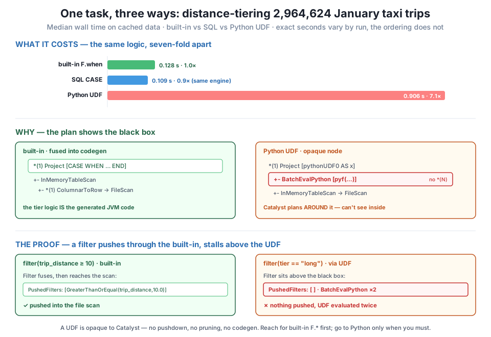
F.when (0.128 s) and SQL CASE (0.109 s) are the same engine and fuse into whole-stage codegen; the Python UDF (0.906 s) is 7.1× slower because every row crosses the JVM-to-Python bridge and the plan shows an opaque BatchEvalPython node Catalyst cannot optimize through. A filter pushes into the scan for the built-in (PushedFilters populated) but stalls above the UDF (PushedFilters: []), which is even evaluated twice. Exact seconds vary by run and machine; the ordering does not.Exercise 1 — Rewrite a UDF as a built-in and measure the win. Suppose a colleague computes fare-per-mile with a Python UDF: F.udf(lambda fare, dist: fare / dist if dist and dist > 0 else None, DoubleType()). Rewrite it as a built-in expression using F.when/F.col, confirm the two produce identical results on the January data, and time both. Report the speedup and find the BatchEvalPython node that disappears from the plan.
Hint
The built-in is F.when(F.col("trip_distance") > 0, F.col("fare_amount") / F.col("trip_distance")), which returns null outside the condition automatically. Compare with df.select(...).filter(F.col("a") != F.col("b")) (guarding for null equality) to confirm agreement, then wrap each in the median_secs harness from this lesson. The built-in plan will show a fused Project; the UDF plan a BatchEvalPython.
Exercise 2 — Prove the double-evaluation costs real time. The blocked-pushdown plan showed BatchEvalPython twice when a filter depended on the UDF’s output. Build two queries that both keep only long trips and count them: one filters on tier_udf("trip_distance") == "long" directly, the other first does .withColumn("tier", tier_udf(...)), then .cache(), then filters. Time both and explain why materializing the UDF column once can beat evaluating it twice.
Hint
Caching forces the UDF to run once and stores the result, so the subsequent filter reads a materialized column instead of re-crossing the bridge. This previews Module 5’s caching — here it’s a concrete case where paying for one UDF pass plus storage beats paying for two passes. Watch the plan change from two BatchEvalPython nodes to an InMemoryTableScan.
Exercise 3 — Find the built-in you didn’t know existed. Data engineers reach for UDFs most often on strings and dates, where a built-in almost always already exists. Take the pickup timestamp and, without any UDF, extract: the hour of day, the day of week name, whether it’s a weekend, and the trip’s duration in minutes. Use only pyspark.sql.functions. Then argue in a comment why a UDF for any of these would be a mistake.
Hint
Look at F.hour, F.date_format(ts, "EEEE"), F.dayofweek (1=Sunday, 7=Saturday), and for duration the cast("timestamp").cast("long") trick from Lesson 1 of Module 3 (the difference is in seconds). Every one of these is a native expression that fuses into codegen and pushes down — a UDF would forfeit all of that to reimplement what the library already provides in the JVM.
You measured the cost of the optimizer’s blind spot. A user-defined function is opaque to Catalyst: it cannot be pushed down, pruned through, simplified, or code-generated, because the engine has no view inside your Python. On 2,964,624 real January trips, classifying by distance tier ran in 0.128 s as a built-in F.when expression and 0.109 s as SQL — the same engine, fused into whole-stage codegen — but 0.906 s as a Python UDF, 7.1x slower, because every value crosses the JVM-to-Python bridge and the plan carries an opaque BatchEvalPython node instead of a fused Project. A filter pushed cleanly into the scan for the built-in (PushedFilters populated) but stalled above the UDF (PushedFilters: []), which Catalyst even evaluated twice when a filter depended on it. The rule that follows is ordered by cost, not preference: built-in functions first; a vectorized pandas_udf when you genuinely need Python and your stack supports Arrow; plain Python UDFs last and small.
BatchEvalPython / ArrowEvalPython — the plan node marking where Spark ships rows to a Python worker. It carries no *(N) codegen marker because it cannot be fused; spotting it tells you a UDF is in the path.F.* first (native, fused, pushable); vectorized pandas_udf when you must use Python and Arrow works on your stack; plain udf last. Performance, and even whether the Arrow path runs, depends on your pandas/Arrow versions.CityFlow’s pipelines will be full of temptations to reach for a UDF — a custom fare rule, a zone-name cleanup, a business classification — and each one quietly switches off the optimizer for that column. On three million rows the difference was seven-fold; on a genuinely large job, or one where the UDF sits before a join or aggregation, it is the difference between a report that lands before the dashboard refresh and one that misses it. The discipline is simple and it pays every time: before writing a UDF, spend thirty seconds looking for the built-in, because it almost always exists and it is always faster. And when a UDF is truly unavoidable, you now know to keep it small, prefer the vectorized form, pin the versions it depends on, and never make the optimizer’s job harder than it already is. That judgment — knowing exactly what you trade away when you drop into Python — is what the next lesson puts to work, fixing a deliberately slow query one plan-diagnosed pathology at a time.
You can now read a plan, recognize what Catalyst optimized, and spot the opaque node where it gave up. Lesson 5, the module’s guided project, hands you a query that is slow on purpose — a Python UDF where a built-in would do, a needless wide projection, a join forced to shuffle, a filter applied too late — and asks you to fix it the way a professional does: not by guessing, but by reading the plan, naming each pathology from the node that reveals it, and repairing them one at a time while the wall-clock time and the plan both improve in front of you. Everything from this module comes together there, and it ends where every good optimization ends — with the fast version producing exactly the same verified answer as the slow one.
Keep DATATWEETS free. Help fund practical data, AI, and engineering lessons for learners worldwide.
