Title here
Summary here
Everything in this module has been preparing you for a single skill: making a slow query fast on purpose, by understanding rather than guessing. You can register a view and write SQL (Lesson 1), read a physical plan node by node (Lesson 2), recognize Catalyst’s optimizations and their limits (Lesson 3), and spot the opaque node where a UDF switches the optimizer off (Lesson 4). This project puts all four to work on one query.
Here is the setup. A colleague at CityFlow has written the zone-hour report — the same report you rebuilt in Module 3, the one that must total $256,692,373.14 across the quarter — but their version is slow. On a single month it takes nearly two minutes; on the full quarter it would be unusable. They ask you to speed it up. You could start rewriting on instinct, but the professional move is different: run it, read its plan, and let the plan tell you exactly what is wrong. Every slow query wears its pathologies openly in its execution plan, if you know how to read them — and you now do.
By the end you’ll have taken a query from 110 seconds to 0.70 seconds on one month — 157 times faster — by fixing four specific things, each diagnosed from a specific plan node, each measured. And the fast version will return byte-identical results to the slow one and reproduce Course 1’s quarter to the cent. The point is not the speedup number; it’s the method, which you’ll keep as a reusable checklist.
By the end of this project, you will be able to:
You’ll need pyspark with its Java runtime. Let’s make a slow query fast.
Before touching the query, write down what “done” means:
The data is New York City’s public-domain Yellow Taxi trip records — the same three months as the rest of the course, plus the zone lookup. Every runnable block below reads the local copies:
# gate: skip
# Fetch once; every block afterward reads the local cached copies by name.
import urllib.request
for m in ("01", "02", "03"):
    urllib.request.urlretrieve(
        f"https://d37ci6vzurychx.cloudfront.net/trip-data/yellow_tripdata_2024-{m}.parquet",
        f"yellow_tripdata_2024-{m}.parquet")
urllib.request.urlretrieve(
    "https://datatweets.com/datasets/nyc-taxi/taxi_zone_lookup.csv", "taxi_zone_lookup.csv")
One session for the whole project. Note the same pythonUDF.arrow.enabled=false line from Lesson 4 — the slow query uses a Python UDF, and on this pandas version the Arrow UDF path deadlocks, so we pin the classic path:
import warnings; warnings.filterwarnings("ignore")
import time, datetime as dt
from pyspark.sql import SparkSession, functions as F
from pyspark.sql.types import TimestampType

spark = (SparkSession.builder
         .appName("cityflow-optimize")
         .master("local[*]")
         .config("spark.ui.showConsoleProgress", "false")
         .config("spark.sql.execution.pythonUDF.arrow.enabled", "false")
         .getOrCreate())
spark.sparkContext.setLogLevel("ERROR")

FILES = ["yellow_tripdata_2024-01.parquet", "yellow_tripdata_2024-02.parquet", "yellow_tripdata_2024-03.parquet"]
JAN = ["yellow_tripdata_2024-01.parquet"]
LO, HI = dt.datetime(2024, 1, 1), dt.datetime(2024, 4, 1)

zones = (spark.read.option("header", True).csv("taxi_zone_lookup.csv")
         .select(F.col("LocationID").cast("int").alias("LocationID"), "Zone", "Borough"))
print("zone dimension rows:", zones.count())
zone dimension rows: 265Here is the colleague’s report. Read it and you can already feel the trouble — but we’ll let the plan confirm every instinct. It extracts the hour bucket with a Python UDF, keeps all nineteen columns through the join, joins the zone dimension with the auto-broadcast turned off (a stand-in for the many real ways a join ends up shuffled — a wrapped key, a type mismatch, a config), and applies the window filter late, after the join.
# gate: skip
# The slow version: a Python UDF for the hour, no column pruning, a forced shuffle join,
# and the window filter applied after the join.
trunc_udf = F.udf(lambda ts: ts.replace(minute=0, second=0, microsecond=0) if ts else None,
                  TimestampType())

def slow_report(files):
    raw = spark.read.parquet(*files)                                  # all 19 columns
    df = raw.withColumn("hr", trunc_udf("tpep_pickup_datetime"))      # UDF for the hour bucket
    joined = df.join(zones, df.PULocationID == zones.LocationID, "inner")   # forced shuffle join
    windowed = joined.filter((F.col("tpep_pickup_datetime") >= F.lit(LO)) &
                             (F.col("tpep_pickup_datetime") <  F.lit(HI)))   # filter, written late
    return windowed.groupBy("PULocationID", "Zone", "hr").agg(
        F.count(F.lit(1)).alias("trips"), F.sum("total_amount").alias("rev"))

spark.conf.set("spark.sql.autoBroadcastJoinThreshold", "-1")   # disable auto-broadcast
slow_report(JAN).count()                                       # warm
start = time.perf_counter(); n = slow_report(JAN).count(); slow_secs = time.perf_counter() - start
print(f"slow: {slow_secs:.2f} s   ({n:,} zone-hour buckets for January)")
slow: 110.17 s (77,533 zone-hour buckets for January)One hundred and ten seconds for a single month. Now the diagnosis — read the plan, don’t guess:
# gate: skip
slow_report(JAN).explain()
== Physical Plan ==
AdaptiveSparkPlan isFinalPlan=false
+- HashAggregate(keys=[PULocationID, Zone, hr], functions=[count(1), sum(total_amount)])
+- HashAggregate(keys=[PULocationID, Zone, hr], functions=[partial_count(1), partial_sum(total_amount)])
+- Project [PULocationID, total_amount, hr, Zone]
+- SortMergeJoin [PULocationID], [LocationID], Inner
:- Sort [PULocationID ASC NULLS FIRST], false, 0
: +- Exchange hashpartitioning(PULocationID, 200), ENSURE_REQUIREMENTS
: +- Project [PULocationID, total_amount, pythonUDF0 AS hr]
: +- BatchEvalPython [<lambda>(tpep_pickup_datetime)], [pythonUDF0]
: +- Filter (... >= 2024-01-01 ... AND ... < 2024-04-01 ... AND isnotnull(PULocationID))
: +- FileScan parquet [tpep_pickup_datetime,PULocationID,total_amount] ... PushedFilters: [IsNotNull(tpep_pickup_datetime), GreaterThanOrEqual(...), LessThan(...)]
+- Sort [LocationID ASC NULLS FIRST], false, 0
+- Exchange hashpartitioning(LocationID, 200), ENSURE_REQUIREMENTS
+- Project [cast(LocationID as int) AS LocationID, Zone]
+- Filter isnotnull(cast(LocationID as int))
+- FileScan csv [LocationID, Zone] ...The plan names three real problems and quietly corrects a fourth:
BatchEvalPython [<lambda>(...)] — the opaque UDF node from Lesson 4. Every one of January’s ~2.96 million pickup timestamps crosses the JVM-to-Python bridge to be truncated. This is the node to suspect first, because a per-row Python call over millions of rows is the single most expensive thing in this plan.SortMergeJoin with two Sorts and two Exchange hashpartitioning(..., 200) — the join shuffles both sides across the network and sorts them, because we disabled the broadcast. The 265-row zone table is tiny; shuffling nine million trips to meet it is pure waste (Module 3, Lesson 3).select("*") habit would carry all nineteen through the exchange. (Here Catalyst’s pruning already trimmed the ReadSchema to the three the query references, but on a genuine select("*") it cannot, and the shuffle balloons.)PushedFilters: [... GreaterThanOrEqual ..., LessThan ...]. Catalyst pushed it all the way down to the file anyway, because it’s a filter on a raw column. This is our first honest lesson: not every “optimization” is yours to make — the optimizer already handles filter placement for raw columns. We’ll confirm this costs nothing to “fix.”Now we repair the query incrementally, timing every step on January and watching the plan change. The order is deliberate — biggest suspect first.
# gate: skip
# Each variant is the same report with one more pathology fixed. Timed on January.
def variant(files, use_udf, prune, broadcast, early):
    raw = spark.read.parquet(*files)
    if prune: raw = raw.select("tpep_pickup_datetime", "PULocationID", "total_amount")
    if early: raw = raw.filter((F.col("tpep_pickup_datetime") >= F.lit(LO)) &
                               (F.col("tpep_pickup_datetime") <  F.lit(HI)))
    df = raw.withColumn("hr", trunc_udf("tpep_pickup_datetime") if use_udf
                              else F.date_trunc("hour", "tpep_pickup_datetime"))
    z = F.broadcast(zones) if broadcast else zones
    joined = df.join(z, df.PULocationID == zones.LocationID, "inner")
    if not early: joined = joined.filter((F.col("tpep_pickup_datetime") >= F.lit(LO)) &
                                         (F.col("tpep_pickup_datetime") <  F.lit(HI)))
    return joined.groupBy("PULocationID", "Zone", "hr").agg(
        F.count(F.lit(1)).alias("trips"), F.sum("total_amount").alias("rev"))

steps = [("0  baseline (udf + wide + SMJ + late filter)", (True,  False, False, False), "-1"),
         ("1  + built-in date_trunc (kill the UDF)",       (False, False, False, False), "-1"),
         ("2  + prune to 3 columns",                       (False, True,  False, False), "-1"),
         ("3  + filter early",                             (False, True,  False, True ), "-1"),
         ("4  + broadcast the zone dimension",             (False, True,  True,  True ), "10485760")]

for label, args, thr in steps:
    spark.conf.set("spark.sql.autoBroadcastJoinThreshold", thr)
    variant(JAN, *args).count()  # warm
    start = time.perf_counter(); variant(JAN, *args).count()
    print(f"{label:44s}: {time.perf_counter() - start:6.2f} s")
0 baseline (udf + wide + SMJ + late filter) : 117.24 s
1 + built-in date_trunc (kill the UDF) : 1.13 s
2 + prune to 3 columns : 1.02 s
3 + filter early : 1.11 s
4 + broadcast the zone dimension : 0.54 sRead that table carefully, because it is the whole lesson in five rows.
The UDF was almost the entire cost. Replacing trunc_udf with the built-in F.date_trunc — one line — took the query from 117.24 s to 1.13 s, a hundred-fold improvement from a single fix. date_trunc is a native expression that fuses into codegen and truncates the hour in the JVM; the UDF shipped three million timestamps to Python and back. Everything else in the query was a rounding error next to that one node. This is why you read the plan first and attack the BatchEvalPython before anything else.
Pruning helped a little; filtering early helped nothing. Trimming to three columns shaved 1.13 to 1.02 s. Writing the filter early moved it from 1.02 back to 1.11 s — no improvement, within noise — exactly as the plan predicted in Step 1: Catalyst was already pushing the raw-column filter to the scan regardless of where we wrote it. A less careful engineer would “fix” the filter placement, see no change, and be confused. You read the plan, expected no change, and got none. Knowing which fixes are already handled for you is as valuable as knowing which are not.
The broadcast join was the second real win. Restoring auto-broadcast flipped the SortMergeJoin to a BroadcastHashJoin and halved the time, 1.11 to 0.54 s — no more shuffling nine million trips to meet 265 rows. Here’s the fast plan, for the same query, confirming both structural wins:
# gate: skip
spark.conf.set("spark.sql.autoBroadcastJoinThreshold", "10485760")
variant(JAN, False, True, True, True).explain()
== Physical Plan ==
AdaptiveSparkPlan isFinalPlan=false
+- HashAggregate(keys=[PULocationID, Zone, hr], functions=[count(1), sum(total_amount)])
+- Exchange hashpartitioning(PULocationID, Zone, hr, 200), ENSURE_REQUIREMENTS
+- HashAggregate(keys=[PULocationID, Zone, hr], functions=[partial_count(1), partial_sum(total_amount)])
+- Project [PULocationID, total_amount, hr, Zone]
+- BroadcastHashJoin [PULocationID], [LocationID], Inner, BuildRight
:- Project [PULocationID, total_amount, date_trunc(hour, ..., Some(Asia/Tehran)) AS hr]
: +- Filter (... >= 2024-01-01 ... AND ... < 2024-04-01 ... AND isnotnull(PULocationID))
: +- FileScan parquet [tpep_pickup_datetime,PULocationID,total_amount] ... PushedFilters: [IsNotNull(...), GreaterThanOrEqual(...), LessThan(...)]
+- BroadcastExchange HashedRelationBroadcastMode(...)
+- Project [cast(LocationID as int) AS LocationID, Zone]
+- Filter isnotnull(cast(LocationID as int))
+- FileScan csv [LocationID, Zone] ...The BatchEvalPython node is gone, replaced by an inline date_trunc expression fused into the Project. The two SortMergeJoin exchanges are gone, replaced by a single BroadcastExchange that ships the tiny zone table to every task — no big-side shuffle. The only remaining Exchange is the group-by’s, which is irreducible: aggregating by key genuinely requires one shuffle. The plan is now as lean as the query allows.
A fast query that returns the wrong answer is a bug with good performance numbers. So we check the optimized report against the slow one (they must be row-identical) and against Course 1’s ground truth (to the cent). First, define the clean final version and confirm it equals the slow one on January:
# gate: skip
def fast_report(files):
    raw = (spark.read.parquet(*files)
           .select("tpep_pickup_datetime", "PULocationID", "total_amount")
           .filter((F.col("tpep_pickup_datetime") >= F.lit(LO)) &
                   (F.col("tpep_pickup_datetime") <  F.lit(HI))))
    df = raw.withColumn("hr", F.date_trunc("hour", "tpep_pickup_datetime"))
    joined = df.join(F.broadcast(zones), df.PULocationID == zones.LocationID, "inner")
    return joined.groupBy("PULocationID", "Zone", "hr").agg(
        F.count(F.lit(1)).alias("trips"), F.sum("total_amount").alias("rev"))

a = slow_report(JAN).select("PULocationID", "hr", "trips", "rev")
b = fast_report(JAN).select("PULocationID", "hr", "trips", "rev")
print("slow and fast are row-identical:", a.subtract(b).count() + b.subtract(a).count() == 0)
slow and fast are row-identical: TrueIdentical — the optimizations changed only how the work runs, never what it computes. Now the real test: run the fast report on the full quarter and check it against the numbers Course 1 established with pandas and multiprocessing. This block is the one the automated check actually runs, because it is fast and it is the claim that matters:
def fast_report(files):
    raw = (spark.read.parquet(*files)
           .select("tpep_pickup_datetime", "PULocationID", "total_amount")
           .filter((F.col("tpep_pickup_datetime") >= F.lit(LO)) &
                   (F.col("tpep_pickup_datetime") <  F.lit(HI))))
    df = raw.withColumn("hr", F.date_trunc("hour", "tpep_pickup_datetime"))
    joined = df.join(F.broadcast(zones), df.PULocationID == zones.LocationID, "inner")
    return joined.groupBy("PULocationID", "Zone", "hr").agg(
        F.count(F.lit(1)).alias("trips"), F.sum("total_amount").alias("rev"))

report = fast_report(FILES).cache()
buckets = report.count()
totals = report.agg(F.sum("trips").alias("t"), F.sum("rev").alias("r")).collect()[0]
print(f"zone-hour buckets : {buckets:,}")
print(f"trips             : {totals['t']:,}")
print(f"revenue           : ${totals['r']:,.2f}")
print("\nbusiest pickup zones over the quarter:")
podium = (report.groupBy("PULocationID", "Zone").agg(F.sum("trips").alias("trips"))
          .orderBy(F.desc("trips")).limit(5).collect())
for r in podium:
    print(f"  {r['PULocationID']:>3}  {r['Zone']:<26} {r['trips']:>9,}")
zone-hour buckets : 240,917
trips : 9,554,757
revenue : $256,692,373.14
busiest pickup zones over the quarter:
161 Midtown Center 453,825
237 Upper East Side South 439,138
132 JFK Airport 429,745
236 Upper East Side North 416,508
162 Midtown East 336,460Exactly right. 240,917 buckets, 9,554,757 trips, $256,692,373.14 to the cent, and the busiest-zone podium to the trip — the same answer Course 1’s capstone produced with a completely different engine, now computed by an optimized Spark query in a fraction of a second. The whole point of the acceptance criteria is met: faster, and provably the same.
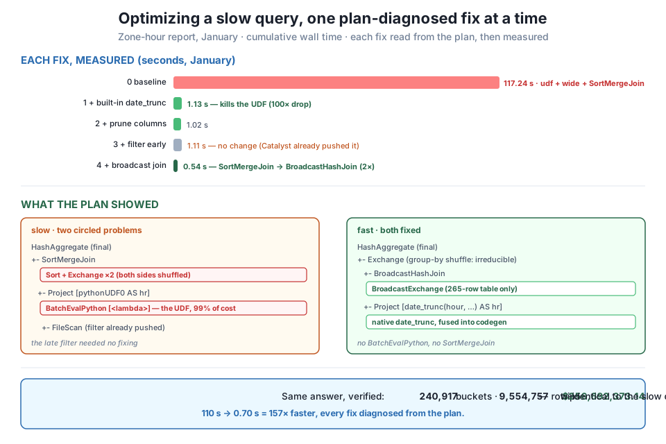
date_trunc alone took it from 117.24 s to 1.13 s — the BatchEvalPython node was 99% of the cost. Restoring the broadcast join (flipping SortMergeJoin to BroadcastHashJoin) halved it again to 0.54 s. Filtering early changed nothing — Catalyst already pushed the raw-column filter to the scan. The optimized report is row-identical to the slow one and reproduces Course 1's quarter exactly: 240,917 buckets, 9,554,757 trips, $256,692,373.14. Exact seconds vary by run; the ordering and the diagnosis do not.The fast query is worth having, but the method is what you keep. When a Spark job is slow, work the plan top to bottom in this order:
.explain() before changing anything. The plan tells you where the time goes; instinct often doesn’t.BatchEvalPython / ArrowEvalPython nodes first. A UDF is usually the single most expensive thing in a plan. Ask whether a built-in F.* function does the same job — it almost always does, and it fused this query’s 117 seconds down to 1.SortMergeJoin with Exchange on both sides, where one side is small, means a broadcast was missed — a wrapped key, a type mismatch, or a disabled threshold. Restore it with broadcast() and watch it become BroadcastHashJoin.ReadSchema for a wide read. If the scan reads columns you never use, prune with an explicit select so they never enter the shuffle.PushedFilters before “fixing” filter placement — Catalyst pushes raw-column filters for you. Don’t spend effort the optimizer already spent.That sequence turned a two-minute query into a half-second one, and every step was a reading of the plan rather than a guess.
Exercise 1 — Isolate the UDF’s share of the cost. The incremental table implies the UDF was almost the entire runtime. Prove it directly: time the slow query, then time a version identical in every way except that trunc_udf is replaced by F.date_trunc — changing nothing else (keep the wide read, the forced SortMergeJoin, the late filter). Report what fraction of the original 110+ seconds the UDF alone accounted for.
Hint
Call variant(JAN, use_udf=True, prune=False, broadcast=False, early=False) and then variant(JAN, use_udf=False, prune=False, broadcast=False, early=False), both with autoBroadcastJoinThreshold=-1. The second should land near 1 s while the first is 100+ s — so the UDF was roughly 99% of the cost, and the SortMergeJoin you left in place is the small remainder.
Exercise 2 — Confirm the filter really is already pushed. Step 1 claimed Catalyst pushes the window filter to the scan even when you write it late. Verify it: take the slow query (filter after the join) and a version with the filter written first, and compare their .explain() output at the FileScan line. Are the PushedFilters identical?
Hint
Look for PushedFilters: [IsNotNull(tpep_pickup_datetime), GreaterThanOrEqual(...), LessThan(...)] in both plans. They should match, because the filter is on a raw column the scan can evaluate — proof that filter placement in your code is not always a real lever. It would matter if the filter depended on the UDF’s output (Lesson 4’s blocked pushdown).
Exercise 3 — Break the broadcast on purpose, then read it. Wrap the join key so the broadcast is defeated: join on df.PULocationID == (zones.LocationID + 0) or cast one side to a different numeric type, and read the plan. Does it fall back to SortMergeJoin? Then fix it and confirm BroadcastHashJoin returns. This is how broadcasts get lost in real code.
Hint
A computed or type-mismatched join key can prevent Spark from recognizing the small side as broadcastable, or force a cast that blocks it. The plan will show SortMergeJoin with two Exchange/Sort pairs instead of BroadcastHashJoin + BroadcastExchange. Match the key types exactly and wrap the small side in broadcast() to restore it — the single most common real-world cause of an accidental shuffle join.
You took a real analytical query from 110 seconds to 0.70 seconds on one month — 157x faster — without guessing once. Reading its plan revealed four issues: an opaque BatchEvalPython UDF computing the hour bucket, a SortMergeJoin shuffling nine million trips to meet a 265-row table, a wide read feeding the shuffle, and a filter written late. You fixed them one at a time and measured each: replacing the UDF with the built-in F.date_trunc alone cut 117.24 s to 1.13 s (the UDF was ~99% of the cost), pruning columns shaved a little more, restoring the broadcast join halved it again to 0.54 s by flipping to BroadcastHashJoin — and filtering early changed nothing, because Catalyst was already pushing the raw-column filter to the scan, a fix that wasn’t yours to make. The optimized report is row-identical to the slow one and reproduces Course 1’s quarter to the cent: 240,917 buckets, 9,554,757 trips, $256,692,373.14. The lasting deliverable is the method — read the plan, attack the opaque node, check the join, prune the read, respect what the optimizer already does, and verify the answer every time.
.explain() output; instinct misleads, the plan does not.BatchEvalPython node over millions of rows dominated everything else; replacing it with a built-in was a 100x fix from one line.SortMergeJoin on a small table is a missed broadcast — two Exchange nodes where one side is tiny means a shuffle you can delete with broadcast(), flipping it to BroadcastHashJoin.PushedFilters first saves wasted effort.CityFlow’s real jobs will arrive slow far more often than they arrive broken, and the instinct to start rewriting on a hunch wastes hours and sometimes makes things worse. The discipline this project teaches — run it, read the plan, fix the biggest diagnosed pathology first, measure, and verify the answer held — is exactly how professional data engineers turn a query that misses the nightly window into one that finishes with room to spare. It scales far past this example: the same .explain() reading that found a UDF and a shuffle join here finds skewed partitions, accidental cartesian products, and unnecessary sorts in jobs a thousand times larger. You’ve now optimized a query the way it’s actually done — not faster because you were lucky, but faster because you understood exactly what was slow and why.
You’ve learned to read what Spark plans and to fix a query by changing the logic it runs — killing a UDF, restoring a broadcast, pruning a read. Module 5, Partitions, Shuffles & Caching, goes one level deeper, to changing the physical execution itself: how many partitions the data is split into, what a shuffle actually costs when it moves data across the network, and when caching a DataFrame pays for itself versus when it just wastes memory. The single irreducible Exchange left in your fast plan — the group-by’s shuffle — is where that story begins, because the next question a performance-minded engineer asks is not “can I avoid this shuffle?” but “how big is it, and can I make it cheaper?” That is Module 5, and it is where Spark tuning stops being about cleaning up the query and starts being about shaping the machine underneath it.
Keep DATATWEETS free. Help fund practical data, AI, and engineering lessons for learners worldwide.
