Lesson 1 - The Ceiling of One Machine

Welcome to The Ceiling of One Machine#

The previous course ended with a result worth being proud of. CityFlow’s pipeline processed the full first quarter of 2024 — 9,554,778 yellow-taxi trips — under a 400 MB memory budget, produced the zone-hour report the dashboard team asked for, and verified the quarter’s revenue to the cent: $256,692,373.14. Every technique in that course pointed the same direction: before you reach for a cluster, use the machine you have well — right dtypes, chunked reads, all ten cores, an index instead of a scan. That argument stands. Nothing in this course retracts it, and the first thing this lesson does is reproduce that verified number on this same laptop, in seconds.

Then it takes the other side, honestly. Every serious data team eventually runs Spark, Snowflake, BigQuery, or something shaped like them — engines that spread one job across many machines — and “the data got big” is not an explanation, it is a slogan. The real explanation is that one machine is one: one set of cores that parallelism can saturate but never exceed, one disk with one throughput and one capacity, one memory ceiling that streaming defers but never removes, and one failure domain for a job that must finish tonight. Those four limits are claims about hardware, so this lesson treats them the way this path treats every claim — by measuring them, on the real taxi quarter, with numbers you can rerun. By the end, the word distributed will be earned rather than assumed, and you will know exactly what an engine has to provide before Lesson 2 shows how Spark provides it.

By the end of this lesson, you will be able to:

• Re-verify Course 1’s ground truth with a parallel zone-hour aggregation — 240,917 buckets and $256,692,373.14 to the cent — and read its speedup curve honestly
• Show by measurement that no worker count exceeds the hardware: 6.86x is the peak, at exactly 10 workers on 10 cores, and 20 workers is worse
• Measure sequential disk throughput around the page cache (~2.7 GB/s uncached) and extrapolate what one disk means for 1 TB and 100 TB
• Explain why streaming defers the memory ceiling but cannot shrink a large answer, using a dedup set that costs a measured 557 MB for one month
• Weigh vertical against horizontal scaling, and state precisely what a distributed engine must provide — and what it will cost

You’ll need pandas, pyarrow, and Python’s standard library (multiprocessing, fcntl, resource). No Spark yet — that is deliberate: this lesson earns the need for it. Let’s find the ceiling.

The Machine That Just Won#

The data is the same public NYC TLC Trip Record Data quarter the previous course verified — January, February, and March 2024. Fetch the three months once and keep them next to your script; every runnable block below reads the local copies by name:

# gate: skip
# CityFlow's verified quarter, fetched once from the public TLC source.
import urllib.request
for month in ("01", "02", "03"):
    name = f"yellow_tripdata_2024-{month}.parquet"
    urllib.request.urlretrieve(
        f"https://d37ci6vzurychx.cloudfront.net/trip-data/{name}", name)

Start by letting the files state their own size — Parquet keeps row counts in its footer metadata, so this costs milliseconds:

import warnings
warnings.filterwarnings("ignore")
import fcntl
import math
import multiprocessing as mp
import os
import resource
import shutil
import statistics
import sys
import time
import pyarrow.parquet as pq

FILES = [
    "yellow_tripdata_2024-01.parquet",
    "yellow_tripdata_2024-02.parquet",
    "yellow_tripdata_2024-03.parquet",
]

if __name__ == "__main__":
    total_rows = 0
    total_bytes = 0
    for path in FILES:
        meta = pq.ParquetFile(path).metadata
        size = os.path.getsize(path)
        total_rows += meta.num_rows
        total_bytes += size
        print(f"{path}: {meta.num_rows:,} rows in {meta.num_row_groups} row groups, {size / 1e6:.0f} MB")
    print(f"the quarter : {total_rows:,} trips, {total_bytes / 1e6:.1f} MB on disk")
    print(f"this machine: {os.cpu_count()} cores")

yellow_tripdata_2024-01.parquet: 2,964,624 rows in 3 row groups, 50 MB
yellow_tripdata_2024-02.parquet: 3,007,526 rows in 3 row groups, 50 MB
yellow_tripdata_2024-03.parquet: 3,582,628 rows in 4 row groups, 60 MB
the quarter : 9,554,778 trips, 160.4 MB on disk
this machine: 10 cores

Nine and a half million trips in 160.4 MB — the quarter that felt enormous in Course 1’s first module now looks almost quaint, which is exactly why it is the right instrument here. Data this small lets us run every experiment in seconds and repeat it until we trust it. The four ceilings we are about to measure do not care how big the input is; they are properties of the machine — this one being a 10-core Apple laptop with 16 GB of RAM and one internal SSD. (You will also notice one block in this lesson wraps its driver code in if __name__ == "__main__": and the next does too — that is Course 1’s spawn rule, and it matters again today: spawned worker processes re-import your script, so worker functions live at top level and everything that runs lives under the guard.)

Ceiling 1: Cores Saturate#

Course 1’s parallel aggregation project ended on a curve: 6 workers over 6 partitions delivered 4.26x, 8 workers delivered 4.33x, and Amdahl’s law explained the plateau — about 8% of that job was irreducibly serial, capping it near 12x however many cores you threw at it. But that experiment left a question open. The plateau appeared where the work ran out (6 partitions), so you never saw the other wall: what happens when work is abundant and you keep adding workers past the machine’s core count?

Today’s job is built to answer that. We rebuild the quarter’s zone-hour report — Course 1’s flagship artifact — as a map-reduce over 30 tasks: each of the quarter’s 10 row groups sliced three ways, so there is always more work than workers. Each task does genuinely CPU-bound Python per row: filter to the quarter’s window, bucket by zone and hour, and accumulate four running values per bucket — trip count, revenue, total minutes, and the sum of squared amounts (the dashboard team wants fare variance per bucket, and $\mathrm{Var}(x) = \mathbb{E}[x^2] - \mathbb{E}[x]^2$ means carrying $\sum x^2$ through the reduce). The worker receives a (path, row_group, slice, n_slices) tuple and reads its own data — Course 1 measured why: one partition pickles to 141 MB as a DataFrame and 50 bytes as a tuple.

WINDOW_START = 1_704_067_200_000_000   # 2024-01-01 00:00 in microseconds
WINDOW_END   = 1_711_929_600_000_000   # 2024-04-01 00:00 in microseconds
US_PER_HOUR  = 3_600_000_000


def report_slice(task):
    """MAP: read your own slice of one row group, build a zone-hour partial in pure Python."""
    path, rg_index, part, n_parts = task
    group = pq.ParquetFile(path).read_row_group(
        rg_index, columns=["PULocationID", "tpep_pickup_datetime",
                           "tpep_dropoff_datetime", "total_amount"])
    lo = group.num_rows * part // n_parts
    hi = group.num_rows * (part + 1) // n_parts
    piece = group.slice(lo, hi - lo)
    zones = piece.column("PULocationID").to_pylist()
    pickups = piece.column("tpep_pickup_datetime").cast("int64").to_pylist()   # microseconds
    dropoffs = piece.column("tpep_dropoff_datetime").cast("int64").to_pylist()
    amounts = piece.column("total_amount").to_pylist()

    buckets = {}
    kept = quarantined = 0
    for zone, pickup_us, dropoff_us, amount in zip(zones, pickups, dropoffs, amounts):
        if WINDOW_START <= pickup_us < WINDOW_END:
            minutes = (dropoff_us - pickup_us) / 60_000_000
            key = (zone, pickup_us // US_PER_HOUR)
            entry = buckets.get(key)
            if entry is None:
                buckets[key] = [1, amount, minutes, amount * amount]
            else:
                entry[0] += 1
                entry[1] += amount
                entry[2] += minutes
                entry[3] += amount * amount
            kept += 1
        else:
            quarantined += 1
    return buckets, kept, quarantined


def merge(partials):
    """REDUCE: combine the small partials; fsum the bucket totals for a stable grand total."""
    merged = {}
    kept = quarantined = 0
    for buckets, k, q in partials:
        kept += k
        quarantined += q
        for key, values in buckets.items():
            entry = merged.get(key)
            if entry is None:
                merged[key] = list(values)
            else:
                for i in range(4):
                    entry[i] += values[i]
    revenue = math.fsum(entry[1] for entry in merged.values())
    return merged, kept, quarantined, revenue


N_SLICES = 3

if __name__ == "__main__":
    tasks = []
    for path in FILES:
        for rg in range(pq.ParquetFile(path).metadata.num_row_groups):
            for part in range(N_SLICES):
                tasks.append((path, rg, part, N_SLICES))
    print(f"{len(tasks)} independent tasks (10 row groups x {N_SLICES} slices)")

30 independent tasks (10 row groups x 3 slices)

Two details are load-bearing. The timestamps are datetime64[us], so cast("int64") yields microseconds — Course 1’s unit trap, and the window constants above are written in the same unit for that reason. And the grand total in merge uses math.fsum over the 240,917 bucket subtotals rather than a plain running float, so the reduce’s answer does not drift with summation order — we are about to check it against a number that is correct to the cent.

Run it serially first — both to set the baseline every speedup is measured against, and to check the answer against Course 1’s ground truth before we trust any parallel version of it:

if __name__ == "__main__":
    serial_times = []
    for _ in range(2):
        start = time.perf_counter()
        partials = [report_slice(t) for t in tasks]
        serial_times.append(time.perf_counter() - start)
    serial_secs = min(serial_times)
    zone_hour, kept, quarantined, revenue = merge(partials)
    print(f"serial runs: {serial_times[0]:.2f} s, {serial_times[1]:.2f} s -> baseline {serial_secs:.2f} s")
    print(f"zone-hour buckets : {len(zone_hour):,}")
    print(f"trips kept        : {kept:,}")
    print(f"trips quarantined : {quarantined}")
    print(f"total revenue     : ${revenue:,.2f}")

serial runs: 16.74 s, 16.16 s -> baseline 16.16 s
zone-hour buckets : 240,917
trips kept        : 9,554,757
trips quarantined : 21
total revenue     : $256,692,373.14

Stop on that output for a moment, because it is this course’s method in miniature. 240,917 buckets. 9,554,757 trips kept, 21 quarantined. $256,692,373.14. Every one of those numbers matches the report Course 1 built with pandas and chunked streaming — different code, different data structures, same answer to the cent. That cross-check discipline is how we will hold Spark to account for the rest of this course: same data, same ground truth, no number taken on faith. (The serial run is timed twice and the baseline takes the better one — the first run pays warm-up costs the comparison shouldn’t.)

Now the sweep. Thirty tasks, so work never runs out — and worker counts that go deliberately past the machine’s 10 cores:

if __name__ == "__main__":
    print(f"{'workers':>7}  {'time (s)':>8}  {'speedup':>8}  {'efficiency':>10}")
    for workers in (1, 2, 4, 8, 10, 16, 20):
        start = time.perf_counter()
        with mp.Pool(processes=workers) as pool:
            partials = pool.map(report_slice, tasks)
        secs = time.perf_counter() - start
        check = merge(partials)
        assert (len(check[0]), check[1], check[2]) == (len(zone_hour), kept, quarantined)
        print(f"{workers:7d}  {secs:8.2f}  {serial_secs / secs:7.2f}x  {serial_secs / secs / workers:10.2f}")
    del partials, check, zone_hour   # free the aggregation before the memory measurement below

workers  time (s)   speedup  efficiency
      1     19.54     0.83x        0.83
      2      8.36     1.93x        0.97
      4      4.27     3.78x        0.95
      8      2.74     5.91x        0.74
     10      2.36     6.86x        0.69
     16      2.53     6.38x        0.40
     20      2.78     5.81x        0.29

Read the table from both ends. One worker is slower than serial (0.83x) — a pool of one buys all of multiprocessing’s spawn-and-pickle overhead and none of its parallelism, exactly as Course 1 measured. Two workers are nearly perfect (1.93x, 97% efficiency). Then the curve bends exactly the way Amdahl predicts, and peaks at 6.86x — at 10 workers, on 10 cores. That is not a coincidence, and what happens next is the entire point of this section: 16 workers is worse (6.38x), and 20 workers is worse still (5.81x). There were 30 tasks — three times more work than at the peak — so this is not Course 1’s “ran out of partitions” plateau. This is oversubscription: more processes than cores means the operating system time-slices them across the same 10 pieces of silicon, adding context switches and extra process startup while adding zero compute. Past the core count, worker counts don’t just stop helping — they cost.

It is worth separating the two ceilings in this curve, because they fail differently. Fit Amdahl’s law, $S(N) = \dfrac{1}{(1 - p) + p/N}$, to the 10-worker point and the parallelizable fraction comes out near $p \approx 0.95$ — which puts this job’s theoretical ceiling around 20x with unlimited cores. Amdahl’s ceiling is a property of the job, and you can engineer against it: shrink the serial fraction, rebalance partitions. The hardware ceiling is a property of the machine, and it is absolute. No worker count, no configuration flag, no library choice makes 10 cores compute like 20. Ten workers used the whole machine; there is nothing left to use. To raise this ceiling you do not need a cleverer pool — you need more machines, plural.

One spawn-hygiene note before moving on, because it changed a number in that table: spawned children re-import this script, so everything they import at module top level, they pay for at every pool creation. This lesson’s blocks import pyarrow.parquet at top level because the workers genuinely need it — but pandas, which only the final measurement in this lesson uses, is imported inside that block’s if __name__ == "__main__": guard, keeping it out of the workers’ startup path. With 20 workers, that one line of discipline is twenty avoided pandas imports per pool.

Ceiling 2: One Disk, One Throughput#

The sweep above was CPU-bound — at its best, ten cores chewed through the quarter’s 160 MB in 2.36 s, about 68 MB/s of Parquet. The disk barely noticed. But make the per-row work cheap — vectorized aggregations, columnar scans, the things engines are good at — and the bottleneck moves to the hardware underneath: one disk, with one sequential throughput. That number decides how fast any scan-shaped job can possibly run on this machine, so it is worth measuring properly.

Measuring it properly is the trick, because the operating system is working against your stopwatch. Every file read passes through the page cache — recently read file pages kept in spare RAM — and the taxi files are certainly in it by now; we have read them a dozen times this lesson. Timing those reads would measure RAM, not disk. So the block below builds a fresh 2 GiB scratch file of os.urandom bytes (incompressible, so a clever drive can’t shortcut it), written and read with the page cache bypassed — F_NOCACHE on macOS, posix_fadvise on Linux — and then reads it warm through the cache for contrast:

CHUNK = 8 * 1024 * 1024          # 8 MB reads
SCRATCH = "c2m1l1_scratch.bin"   # namespaced scratch file, deleted below


def bypass_page_cache(fd):
    if hasattr(fcntl, "F_NOCACHE"):                        # macOS
        fcntl.fcntl(fd, fcntl.F_NOCACHE, 1)
    elif hasattr(os, "posix_fadvise"):                     # Linux
        os.posix_fadvise(fd, 0, 0, os.POSIX_FADV_DONTNEED)


def timed_read(path, uncached):
    fd = os.open(path, os.O_RDONLY)
    if uncached:
        bypass_page_cache(fd)
    start = time.perf_counter()
    nbytes = 0
    while True:
        chunk = os.read(fd, CHUNK)
        if not chunk:
            break
        nbytes += len(chunk)
    secs = time.perf_counter() - start
    os.close(fd)
    return nbytes / 1e6 / secs   # MB/s


if __name__ == "__main__":
    block = os.urandom(CHUNK)    # incompressible bytes, so the drive can't cheat
    fd = os.open(SCRATCH, os.O_WRONLY | os.O_CREAT | os.O_TRUNC)
    bypass_page_cache(fd)
    start = time.perf_counter()
    for _ in range(256):         # 2 GiB
        os.write(fd, block)
    os.fsync(fd)
    write_mbs = 256 * CHUNK / 1e6 / (time.perf_counter() - start)
    os.close(fd)
    print(f"sequential write, uncached : {write_mbs:,.0f} MB/s")

    uncached_runs = [timed_read(SCRATCH, uncached=True) for _ in range(3)]
    print("sequential read, uncached  :", "  ".join(f"{r:,.0f} MB/s" for r in uncached_runs))
    timed_read(SCRATCH, uncached=False)                    # populate the page cache
    warm_runs = [timed_read(SCRATCH, uncached=False) for _ in range(2)]
    print("sequential read, page cache:", "  ".join(f"{r:,.0f} MB/s" for r in warm_runs))
    os.remove(SCRATCH)

    disk_mbs = statistics.median(uncached_runs)
    print(f"\nat {disk_mbs:,.0f} MB/s, one full sequential pass takes:")
    for label, mb in (("the quarter", total_bytes / 1e6), ("1 TB", 1e6), ("100 TB", 1e8)):
        secs = mb / disk_mbs
        pretty = (f"{secs:.2f} s" if secs < 60
                  else f"{secs / 60:.1f} min" if secs < 3600
                  else f"{secs / 3600:.1f} h")
        print(f"  {label:12s}: {pretty}")
    print(f"and this disk holds {shutil.disk_usage('.').total / 1e12:.2f} TB in total")

sequential write, uncached : 964 MB/s
sequential read, uncached  : 2,648 MB/s  3,051 MB/s  2,726 MB/s
sequential read, page cache: 4,644 MB/s  3,157 MB/s

at 2,726 MB/s, one full sequential pass takes:
  the quarter : 0.06 s
  1 TB        : 6.1 min
  100 TB      : 10.2 h
and this disk holds 0.49 TB in total

The disk itself is genuinely fast — around 2.7 GB/s of sequential read, which is why Course 1 could afford to re-read partitions instead of shipping them between processes. The extrapolation is where the ceiling appears, and it appears twice. First, throughput: at 2.7 GB/s, one pass over 1 TB is a six-minute wait, and one pass over 100 TB is 10.2 hours — for a single sequential read, the absolute best case, before a byte is decompressed, parsed, or aggregated, and real pipelines read their data many times. Second, and more brutally, capacity: this disk holds 0.49 TB. The 100 TB dataset does not scan slowly on this machine — it does not fit, by a factor of two hundred. There is no software fix for either number. But notice what the arithmetic invites: ten machines, each holding a tenth of the data on its own disk, read at an aggregate 27 GB/s — and that six-minute terabyte becomes thirty-seven seconds. Reading in parallel from many disks is precisely what distributed file systems and object stores exist to make possible, and Spark is built to exploit it.

Ceiling 3: Memory — Deferred, Not Removed#

Course 1’s proudest trick was making memory stop mattering: stream the input in chunks, keep only running aggregates, and the same job that materialized 1,347 MB in pandas ran in a flat few hundred. But that trick has a precondition nobody says out loud, and it is time to say it: streaming keeps memory flat only when the answer is small. The zone-hour report compresses 9,554,778 trips into 240,917 buckets — the input is forty times bigger than the answer, so the input can flow through and be forgotten. Now pose a question whose answer is not small: which distinct trips exist? — the dedup problem from Course 1’s dicts-and-sets lesson. Every arriving key must be checked against every key seen so far, which means the answer itself — the set of distinct keys — must live somewhere, all of it, all the time. Streaming the input changes nothing: the chunks flow through, and their keys pile up. Measure what that answer costs for a single month:

MB = 1024 * 1024   # ru_maxrss is reported in bytes on macOS
KEY_COLS = ["VendorID", "tpep_pickup_datetime", "tpep_dropoff_datetime",
            "PULocationID", "DOLocationID"]

if __name__ == "__main__":
    import pandas as pd   # imported here so spawned workers above never pay for it

    peak_before = resource.getrusage(resource.RUSAGE_SELF).ru_maxrss / MB
    trips = pd.read_parquet(FILES[0], columns=KEY_COLS)
    distinct = set(zip(
        trips["VendorID"].tolist(),
        trips["tpep_pickup_datetime"].astype("int64").tolist(),   # microseconds
        trips["tpep_dropoff_datetime"].astype("int64").tolist(),
        trips["PULocationID"].tolist(),
        trips["DOLocationID"].tolist(),
    ))
    peak_after = resource.getrusage(resource.RUSAGE_SELF).ru_maxrss / MB
    container = sys.getsizeof(distinct)
    tuples = sum(sys.getsizeof(t) for t in distinct)
    stamps = sum(sys.getsizeof(t[1]) + sys.getsizeof(t[2]) for t in distinct)
    retained = (container + tuples + stamps) / 1e6
    print(f"distinct keys, January   : {len(distinct):,}")
    print(f"set container            : {container / 1e6:.2f} MB")
    print(f"+ key tuples             : {tuples / 1e6:.2f} MB")
    print(f"+ timestamp integers     : {stamps / 1e6:.2f} MB")
    print(f"= retained by the answer : {retained:,.0f} MB")
    print(f"peak RSS before -> after : {peak_before:,.0f} MB -> {peak_after:,.0f} MB")

    per_key = retained * 1e6 / len(distinct)
    print(f"\n~{per_key:.0f} bytes per key -- arithmetic from here, not measurement:")
    for label, n in (("the quarter", 9_554_778),
                     ("a year at 2024's pace", 4 * 9_554_778),
                     ("ten years at that pace", 40 * 9_554_778)):
        print(f"  {label:23s}: ~{n * per_key / 1e9:.1f} GB just to hold the answer")

distinct keys, January   : 2,933,515
set container            : 134.22 MB
+ key tuples             : 234.68 MB
+ timestamp integers     : 187.74 MB
= retained by the answer : 557 MB
peak RSS before -> after : 568 MB -> 1,203 MB

~190 bytes per key -- arithmetic from here, not measurement:
  the quarter            : ~1.8 GB just to hold the answer
  a year at 2024's pace  : ~7.3 GB just to hold the answer
  ten years at that pace : ~72.5 GB just to hold the answer

The numbers agree with Course 1 down the line: 2,933,515 distinct keys for January, a 134.22 MB set container (the same figure the dicts-and-sets lesson measured), and once you count what the container points at — 234.68 MB of key tuples and 187.74 MB of timestamp integers (the vendor and zone ids are mostly interned small ints, so this decomposition slightly undercounts) — the answer retains about 557 MB for one month. The process’s high-water mark jumped from 568 MB to 1,203 MB building it, transients included; Course 1’s guided project measured the same probe at 718 MB peak and cut the dedup set from the design for exactly this reason — it was the one structure bounded by rows rather than by anything small.

Then the arithmetic takes over, at a measured ~190 bytes per key: the quarter needs ~1.8 GB, a year at 2024’s pace ~7.3 GB — nearly half this machine’s 16 GB, just to hold the answer — and ten years needs ~72.5 GB, which no amount of streaming discipline fits into 16. Be precise about what one machine can still do here, because the honest answer is “more than you’d think, slower than you’d like”: Course 1’s toolkit defers this ceiling too — spill the keys to disk and sort-merge them, or push them into SQLite and let its B-tree do the work. Those are real techniques and they genuinely work into the tens of gigabytes. But every deferral trades memory for the disk you just measured, pays in wall-clock time, and lands on the same 0.49 TB, 2.7 GB/s device. The ceiling moves; it never leaves. When the answer outgrows the machine, the only move left is to make it several machines’ answer — split the key space so each machine owns a fraction of the keys, all of them, exclusively. Hold that thought; Exercise 3 makes you work it out, and this course will spend whole lessons on what it costs (its name, when Spark does it, is a shuffle).

Ceiling 4: One Failure Domain#

The fourth ceiling never shows up in a benchmark, because it is about the runs that don’t finish. Take the 10.2-hour number from Ceiling 2 — the floor for one pass over 100 TB on this hardware, before any real work — and now let the machine hiccup at hour nine. A kernel panic, a forced OS update, a power cut, a disk that picks today to die. On one machine, the probability of any of these on a given day is small; the consequence is total. The job restarts from zero — or from your last checkpoint, if you built checkpointing by hand the way Course 1’s capstone did — but either way, on the same machine, after you have repaired or rebooted it, with the deadline gone. There is no second machine to pick the work up, because “the machine” and “the system” are the same thing. That identity is what failure domain means: the blast radius of one failure is the entire pipeline.

Checkpoints deserve their honest due here, because they are the single-machine mitigation and they are not nothing: checkpoint every hour and the crash at hour nine costs you one hour of recompute instead of nine. But look at what they do and don’t fix. They shorten the replay; they do nothing for the repair — the job still waits, potentially until tomorrow, for this one box to be healthy again. And hand-rolled checkpointing is exactly the kind of bookkeeping that quietly grows bugs: partial files, half-written state, the checkpoint that didn’t flush before the power went.

Now flip the perspective, because the distributed version of this story is worse in one way and better in every other. A cluster of 200 machines has roughly 200 times the hardware failures — at that scale, something is always broken, and pretending otherwise is not an option. That is precisely why engines built for clusters treat a dying worker as a routine event rather than a catastrophe: the work is already split into small tasks, the engine knows which tasks the dead machine owned, and it reschedules them onto healthy machines while the job keeps running. The job finishes minutes late, not days late, and nobody gets paged. Failure tolerance is not a bonus feature of distributed engines — it is a requirement forced on them by their own scale, and one machine’s design simply never forces anyone to build it.

Bigger Machine, or More Machines?#

Four measured ceilings, one obvious retort: buy a bigger machine. Take it seriously, because it is often right. Vertical scaling — more cores, more RAM, more disk in one box — is the straight continuation of Course 1’s philosophy: no new failure modes, no new code, every technique you know keeps working. A workstation with 32 cores, 256 GB of RAM, and 8 TB of fast storage would lift every number in this lesson by nearly an order of magnitude, and for CityFlow’s actual quarter it would be comfortable overkill.

But follow the road to its end. Each doubling costs more than the last — commodity parts stop being commodity somewhere past the workstation tier, and the top of the vertical road is a machine priced like a house with core counts in the low hundreds and RAM in the low terabytes. Those are 10-to-100-times improvements over this laptop, bought at far worse than 10-to-100-times the price — and every ceiling in this lesson is still there, just higher up: the cores still saturate, the storage still has finite throughput, the dedup answer still eventually outgrows the RAM, and it is still one failure domain; the biggest machine money can buy still reboots for a kernel update with your job nine hours in. Vertical scaling raises the numbers. It never fixes the oneness.

Horizontal scaling attacks the oneness directly: ten ordinary machines instead of one extraordinary one. The arithmetic is immediate — 100 cores, 160 GB of aggregate RAM, ten disks reading in parallel at ~27 GB/s, and any single machine can die without taking the system with it — and the cost curve is linear: the eleventh machine costs the same as the tenth. What it buys you at the high end, nothing vertical can: there is no single machine equivalent to two hundred of these, at any price.

What it costs is the honest half of the bargain, and it is the theme of this entire course: coordination. The data must be partitioned — split across machines, with the system knowing which machine holds what. The work must be scheduled — matched to machines, ideally the machine already holding the data, since Ceiling 2 taught you what moving bytes costs. Partial results must be combined across a network that is slower than RAM by orders of magnitude. And failures must be survived mid-job. Here is the encouraging part: you have already done every one of these things, by hand, at laptop scale, in this very lesson. The 30 slice-tasks were partitions. pool.map was a scheduler. merge() combined partials that — because this was one machine — never had to cross a network. The one you haven’t done is surviving a worker’s death, and you saw why: on one machine, the dying worker takes the whole job with it. A distributed engine is this lesson’s map-reduce grown up: same shape, many machines, plus the machinery that moves partials across a real network and replays lost tasks — done by something that is not you, hand-rolling it per job.

Where Spark Enters#

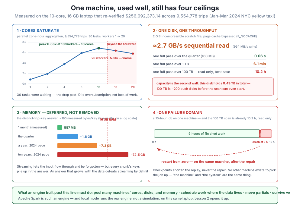
Line the four ceilings up and read them as a job description. Wanted: an engine that treats many machines’ cores as one pool of parallelism (Ceiling 1), reads from many disks at once and schedules work where the data already lives (Ceiling 2), holds large working sets in many machines’ memory and spills with discipline when even that runs out (Ceiling 3), and treats a dying worker as a scheduling event rather than a catastrophe (Ceiling 4) — while letting you describe the what (the same zone-hour report you have now built twice) without hand-rolling the how (partitioning, scheduling, moving partials, replaying lost work) for every job. Apache Spark is that engine, and it is the one this course teaches.

What makes Spark the right classroom, though, is a property this course will lean on in every single lesson: local mode. Spark on your laptop is not a toy, a simulator, or a compatibility layer — it is the genuine engine, the same driver, the same optimizer, the same DataFrame API and execution plans that run on thousand-node clusters, with your 10 cores standing in for a cluster’s workers. Code written against it moves to a real cluster by changing a connection string. That means everything you measure in the next four lessons is real Spark behavior, verifiable against the ground truth this lesson just reproduced — including, in Lesson 4, the measurement most courses skip: the JVM startup, planning, and per-job overhead that make Spark genuinely slower than pandas on small data. A 160 MB quarter does not need a distributed engine, and you now have the numbers to say precisely why — and precisely when that stops being true.

Practice Exercises#

Exercise 1 — Find your own machine’s knee. The sweep jumped from 4 to 8 to 10 workers. Rerun it at every count from 1 to 12 (reuse report_slice, merge, and the 30 tasks), print the same time/speedup/efficiency table, and identify where efficiency first drops below 0.75. Compare the location of the peak against your os.cpu_count(). If your machine has performance and efficiency cores (most modern laptops do), explain which feature of your curve reveals that.

Exercise 2 — The disk arithmetic that justifies a cluster. Using your own measured uncached throughput from the disk block, compute (a) the time for one sequential pass over 10 TB on your machine, and (b) the minimum number of machines — each contributing your measured rate from its own disk — needed to scan those 10 TB in under 60 seconds. Then write down the two assumptions your answer to (b) silently makes, and one sentence each on why they are the hard part.

Exercise 3 — Where exactly does the answer die? Extend the memory measurement: build the distinct-key set for January, then January+February, then the full quarter, recording retained megabytes and keys at each step. Confirm bytes-per-key stays near ~190, then compute how many months of 2024-pace data your machine’s RAM could hold before the answer alone exceeds it. Finally, explain in two or three sentences why splitting the keys across 10 machines by hash(key) % 10 keeps the global dedup exact — no key missed, none double-counted — while each machine holds only a tenth of the answer.

Summary#

You measured the four ceilings of the machine that won Course 1. First, its cores: the zone-hour report rebuilt as a 30-task map-reduce reproduced ground truth exactly — 240,917 buckets, 9,554,757 trips kept, 21 quarantined, $256,692,373.14 to the cent — in 16.16 s serially, and the worker sweep peaked at 6.86x at exactly 10 workers on 10 cores, with 16 workers (6.38x) and 20 workers (5.81x) measurably worse despite three tasks per worker still being available: past the core count, oversubscription costs and nothing pays. Amdahl’s fit put this job’s theoretical ceiling near 20x — unreachable, because the $N$ in the formula stops at the hardware. Second, its disk: a measured ~2.7 GB/s uncached sequential read means 0.06 s for the 160 MB quarter, 6.1 minutes per terabyte, and 10.2 hours per 100 TB — a dataset this 0.49 TB disk could not store at one two-hundredth scale. Third, its memory: the distinct-trip-key answer retained a measured 557 MB for one January (2,933,515 keys at ~190 bytes each; peak RSS 568 → 1,203 MB building it), and the arithmetic passes 16 GB somewhere between a year (~7.3 GB) and ten (~72.5 GB) — streaming defers the input’s memory, never the answer’s. Fourth, its failure domain: one machine is one blast radius, where checkpoints shorten the replay but never the repair. Vertical scaling raises all four numbers without fixing the oneness; horizontal scaling fixes the oneness at the price of coordination — partitioning, scheduling, moving partials, surviving failure — which is the price this course exists to examine, using an engine whose local mode runs the real thing on this same laptop.

Key Concepts#

• Core saturation — parallelism approaches the machine’s core count and never exceeds it: 6.86x at 10 workers on 10 cores was the peak, and 20 workers dropped to 5.81x with work still available. Oversubscription adds context switches, not silicon.
• Amdahl’s ceiling vs the hardware ceiling — $S(N) = 1/((1-p) + p/N)$ caps this job near 20x at $p \approx 0.95$ — a property of the job you can engineer against; the hardware caps $N$ itself at 10 — a property of the machine you cannot.
• One disk, two walls — throughput (~2.7 GB/s measured → 10.2 h per pass over 100 TB) and capacity (0.49 TB): past a size, data doesn’t scan slowly on one machine — it doesn’t fit at all. Ten disks reading in parallel is the move no single disk can match.
• Answer-bounded memory — streaming keeps memory flat only when the answer is small. A dedup answer at ~190 measured bytes/key grows with the data (557 MB/month → ~72.5 GB/decade) and defeats streaming by definition; spill-to-disk defers it again, onto the disk from ceiling two.
• Failure domain — the blast radius of one failure. On one machine it is the whole pipeline: restart from zero (or last checkpoint) on the same box, after the repair. Distributed engines must treat worker death as routine scheduling — their scale forces failures to be normal, not exceptional.

Why This Matters#

CityFlow’s team is about to adopt Spark, and this lesson is the difference between adopting it for reasons and adopting it for fashion. The reasons are now numbers: the exact speedup where the laptop’s cores gave out, the exact hours a single disk would need for the fleet sizes CityFlow’s partners keep mentioning, the exact month count at which a dedup answer eats the RAM, and the one failure that undoes a night of work. Just as important, the same numbers defend the other decision: the quarter is 160 MB, the laptop re-verified a quarter-billion dollars of revenue on it in seconds, and nothing that small justifies a cluster’s coordination tax — a judgment Lesson 4 will sharpen by measuring Spark losing to pandas on exactly this data. Engineers who skip this measuring end up in one of two failure modes: the team that runs a 40-machine cluster to process gigabytes, paying the shuffle tax on data a laptop would crush; or the team that white-knuckles a 30-hour single-machine job through its third overnight crash, because “our data isn’t that big” was last checked two years ago. The map of where one machine ends is what keeps you off both paths — and you now hold a measured copy of it.

Continue Building Your Skills#

You now know why an engine built past the ceiling has to exist, and you know its job description by heart: pool many machines’ cores, read many disks at once, schedule work where data lives, survive dying workers. What you have not seen is how any of that is organized — and that is Lesson 2, Driver, Executors & Local Mode. You’ll meet Spark’s division of labor: a driver that plans the work and holds the job’s brain, executors that do the work and hold the data, and the job → stage → task decomposition that turns one query into schedulable pieces — the industrial version of the tasks you hand-built for pool.map today. Then the part that makes this course possible: how local[*] maps that whole architecture onto your 10 cores, why it is the real engine rather than a simulation, and how to watch it think in the Spark UI at localhost:4040. You’ll inspect a live SparkSession’s master, parallelism, and scheduler for real, on the same machine whose ceilings you just measured — and from there, the course starts putting the quarter through the engine.