Title here
Summary here
You have already built Spark’s architecture once, by hand. In the previous course’s multiprocessing module, a parent process split CityFlow’s taxi data into partitions, handed them to a pool of workers, collected partial results, and merged them — the map-reduce shape that took a 9.60 s job to 2.42 s across six cores. You wrote the coordinator, you wrote the workers, and you wrote the merge. Spark is that same shape, industrialized: the coordinator gets a name (the driver), the worker pool gets a name (the executors), and everything you glued together manually — splitting the work, scheduling it onto cores, surviving a worker’s death, merging the answers — becomes the engine’s job instead of yours. Lesson 1 established why this matters: one machine’s cores saturate, and past that ceiling the work has to spread across machines that share nothing but a network.
This lesson gives you Spark’s mental model — the cast of processes and the hierarchy of work they share — with one goal: that you can predict what Spark will do before it does it. That claim gets tested immediately, because nothing here stays theoretical. You will start a real SparkSession and interrogate it: what master is it running, how many cores does it see, where is its web UI. You will run one aggregation over January’s 2,964,624 real trips and pull out its actual anatomy — how many jobs, how many stages, how many tasks — from Spark’s own status tracker. You will walk into a genuine trap (getOrCreate() handing you back a session you thought you had reconfigured) on purpose, so it never catches you by accident. And you will change exactly one string — local[*] to local[2] — and measure what it does to the same job on the same 9,554,778-trip quarter. Everything runs on your laptop, and none of it is a simulation: local mode is the real engine, which is precisely why it is worth learning this way.
By the end of this lesson, you will be able to:
local[*] runs the real engine rather than a simulation, and what the one-string change to a cluster actually changessc.master, defaultParallelism, the Spark UI on port 4040, and per-job stage/task anatomy from the status trackergetOrCreate() trap, and measure what local[2] versus local[*] does to both partitioning and runtimeYou’ll need pyspark (with a JDK 17 or 21 installed — see the course setup) and the three taxi-quarter Parquet files. Let’s meet the cast.
Every Spark application, from your laptop to a thousand-node cluster, has the same three roles.
The driver is the process your Python code runs in. When you build a SparkSession, you are standing in the driver. It does the thinking: it holds the SparkSession, turns your DataFrame code into a logical plan, hands that plan to the Catalyst optimizer to be rewritten into something efficient, splits the physical plan into stages, and schedules individual tasks onto whatever workers exist. It also collects final results — which is why “bring everything to the driver” will become a memory hazard in Lesson 3. In Course 1’s terms, the driver is the parent process that owned the Pool, decided the partitioning, and did the final merge — except this parent also employs a query optimizer and a scheduler you didn’t have to write.
The executors are the muscle: JVM processes that hold partitions of your data in their memory and run tasks — small units of computation — against them. Each executor has a number of task slots (roughly, cores), executes whatever the driver schedules onto it, and reports back. Executors are Course 1’s worker pool, with two upgrades. First, they keep data resident between steps, so a multi-step pipeline doesn’t re-read its input from disk at every stage the way each new Pool job did. Second, they are replaceable: if an executor dies mid-job, the driver knows which partitions it was responsible for and reschedules just those tasks elsewhere. Your Course 1 pipeline restarted from zero if a worker was killed; Spark’s lineage-based recovery is one of the things that makes a 500-machine job survivable, because at that scale something is always failing.
The cluster manager is the landlord: it owns the machines and leases them out. When a driver says “I need 40 executors with 8 GB each,” the cluster manager (YARN, Kubernetes, or Spark’s own standalone manager) finds room and starts them. It allocates resources; it never sees your data or your plan. On a laptop there is nothing to lease, so in local mode this role collapses to almost nothing — one reason local Spark starts in seconds rather than minutes.
Where your Python actually runs
PySpark is a Python API to a JVM engine. Your script is a Python process, but it drives a JVM that hosts the actual planner, and DataFrame operations — filters, joins, aggregations — compile down to JVM code that runs entirely inside the executors. No trip data flows through Python when you run df.groupBy(...).count(); Python only describes the plan and receives the result. This is why PySpark’s DataFrame API costs almost nothing over Scala’s, and why the picture changes the moment you write a Python UDF — then executors must ship rows out to Python workers and back. That cost gets measured later in the course; for now, know which side of the bridge your code stands on.
The cast shares a vocabulary for work, four levels deep. It is worth learning precisely, because the Spark UI, every log line, and every performance conversation you will ever have about Spark is phrased in it.
An application is everything one SparkSession does from creation to stop() — the whole program. Yours will be called cityflow.
A job is what one action triggers. DataFrame operations come in two kinds: transformations (filter, groupBy, select) describe work but run nothing, while actions (count, collect, show, write) demand an answer and force execution. Call three actions, get at least three jobs. Lesson 3 puts this laziness to work; today it explains where jobs come from.
A stage is a run of work that can proceed without moving rows between partitions. A filter reads a partition and writes a smaller one — no movement, same stage. But groupBy("PULocationID") needs every row for zone 132 in one place, and those rows start out scattered across all partitions; regrouping them is a shuffle, and a shuffle is where Spark cuts the plan into stages: everything before the regrouping is one stage, everything after is another. Shuffles are the single most expensive thing a distributed engine does, and Module 5 is devoted to them; for now you only need the boundary rule — stages end where data must move.
A task is one stage’s work applied to one partition — the atom of scheduling. A stage over a 10-partition DataFrame is 10 tasks; each task runs on one core of one executor. This gives you the prediction rule this lesson promised: tasks per stage = partitions, so if you know how your data is partitioned, you know what Spark will schedule before it schedules it. We are about to check that rule against reality.
Here is the claim that makes this whole course honest: the Spark you run on a laptop is not a toy, a simulator, or a “lite” edition. It is the same engine, told to play every role itself.
The master URL you pass at session-build time tells the driver where its executors will come from. spark://host:7077 says “ask that standalone cluster.” local[*] says “no cluster — run executor threads inside my own JVM, one per core.” local[4] pins it to four threads; local[1] gives you a single-threaded Spark, which sounds useless but is a superb debugging tool. In local mode the driver and the executor share one JVM, the cluster manager has nothing to do, and the “network” between workers is a memory copy. Everything else — the Catalyst optimizer, the physical planner, the stage-cutting, the task scheduler, the shuffle machinery, the UI — is byte-for-byte the code a thousand-node cluster runs.
The consequence cuts both ways, and both directions matter. Forward: code you write and understand this way moves to a real cluster by changing one string, because the plans Spark builds are the same plans. Backward: every behaviour you measure locally — partition counts, stage boundaries, task anatomy, optimizer choices — is real Spark behaviour, not an approximation of it. When this lesson counts 10 tasks in a scan stage, a cluster reading the same files would count the same 10; the difference is whose cores they land on. Local mode does hide one big cost, and we will name it honestly at the end of the lesson — but what it shows you, it shows you truthfully.
Time to stop describing the engine and start it.
The data is the same real quarter Course 1 verified — the public NYC TLC Trip Record Data, January through March 2024. Fetch the three months once and keep them next to your script:
# gate: skip
# CityFlow's verified quarter, fetched once from the public TLC source.
import urllib.request
for month in ("01", "02", "03"):
    urllib.request.urlretrieve(
        f"https://d37ci6vzurychx.cloudfront.net/trip-data/yellow_tripdata_2024-{month}.parquet",
        f"yellow_tripdata_2024-{month}.parquet",
    )
Now build the session. This block is the standard opening for every lesson in this course, and each line earns its place: appName is how you’ll recognise this application in the UI, master("local[*]") is the one-string cluster decision we just discussed, the showConsoleProgress config stops stage progress bars from stomping over your printed output, and setLogLevel("ERROR") silences the WARN chatter (you may still see a warning or two while the JVM boots — harmless).
import warnings
warnings.filterwarnings("ignore")
import time
import statistics
from pyspark.sql import SparkSession
import pyspark.sql.functions as F

t0 = time.perf_counter()
spark = (SparkSession.builder
         .appName("cityflow")
         .master("local[*]")
         .config("spark.ui.showConsoleProgress", "false")
         .getOrCreate())
spark.sparkContext.setLogLevel("ERROR")
print(f"SparkSession up in {time.perf_counter() - t0:.1f} s")
SparkSession up in 6.8 sNotice what those seconds bought: a JVM launched, an executor’s worth of task slots created, a scheduler and an optimizer initialised, a web server started. The exact figure moves with your machine and its load — this one was also running an editor and a browser — but it is never zero, and pd.read_parquet costs none of it, which is a fact Lesson 4 will make Spark answer for. For now, the session is alive — so ask it who it is. The SparkContext (reachable as spark.sparkContext, conventionally sc) is the lower-level handle that knows about the machinery:
sc = spark.sparkContext
print("master             :", sc.master)
print("appName            :", sc.appName)
print("Spark version      :", spark.version)
print("defaultParallelism :", sc.defaultParallelism)
print("Spark UI           :", sc.uiWebUrl)
master : local[*]
appName : cityflow
Spark version : 4.2.0
defaultParallelism : 10
Spark UI : http://localhost:4040Four facts and an address. master confirms the deal we asked for; defaultParallelism is what local[*] resolved to on this machine — 10, one task slot per core, and the number Spark will use as its default answer to “how many pieces should I cut work into?” And uiWebUrl is not a metaphor: your session is running a real web server. Spark printed this machine’s network address; on yours it may say localhost or your machine’s name, and either way http://localhost:4040 reaches it. Open it in a browser now, while the session is alive, and leave the tab open — we are about to put things in it.
The Spark UI is the single most useful debugging tool you will get in this course. Along its top bar: Jobs lists every job the application has run, with its stages and timing; click into a stage and you get a task-level timeline showing exactly which cores did what, when, and for how long. Stages shows the same data stage-first. Storage lists cached data — empty until you learn .cache() later in the course. Environment is every config the session resolved, useful when you suspect a setting didn’t take (foreshadowing). Executors shows the worker pool — in local mode, one entry named driver, because one JVM is playing both parts. And the SQL / DataFrame tab shows each query’s optimized plan, which a later module will teach you to read.
The UI lives and dies with the session
Port 4040 is served by your driver process, so the UI exists exactly as long as the session does — spark.stop() (or your script ending) takes it down, which is why you browse it during a run, not after. If a second Spark application starts while the first holds 4040, it doesn’t fail; it takes 4041, and the next 4042. Check the printed uiWebUrl rather than assuming, and if your script finishes too fast to look around, drop input("UI open — press Enter to finish") before spark.stop().
The hierarchy section made a prediction: tasks per stage equals partitions. Load January and get both numbers:
jan = spark.read.parquet("yellow_tripdata_2024-01.parquet")
print("input partitions :", jan.rdd.getNumPartitions())

t0 = time.perf_counter()
n = jan.count()
print(f"rows             : {n:,}  (counted in {time.perf_counter() - t0:.2f} s)")
input partitions : 10
rows : 2,964,624 (counted in 0.56 s)Two things to bank. The row count is 2,964,624 — exactly the January figure Course 1 established and verified, which is the cross-check discipline this course will apply throughout: same data, new engine, answers must agree. And the 48 MB file came in as 10 partitions: Spark noticed defaultParallelism is 10 and cut the file into ten byte ranges so that every core gets work. Nobody asked it to; keeping all cores busy is the engine’s default posture.
So the prediction is: a job over jan should schedule stages of 10 tasks. Let’s run a real aggregation — January’s busiest pickup zones — and then, instead of guessing what happened, pull the anatomy out of Spark’s status tracker, the same bookkeeping the UI reads. Tagging the work with a job group makes it easy to find:
sc.setJobGroup("anatomy", "top pickup zones, January")
top3 = (jan.groupBy("PULocationID").count()
           .orderBy(F.desc("count")).limit(3).collect())
sc.setJobGroup(None, None)
for row in top3:
    print(f"zone {row['PULocationID']}: {row['count']:,} trips")
zone 132: 145,240 trips
zone 161: 143,471 trips
zone 237: 142,708 tripsPause on the values before the machinery: JFK Airport (132) with 145,240 pickups, Midtown Center (161) with 143,471, Upper East Side South (237) with 142,708 — Course 1’s verified January answer to the trip. The engine changed; the truth didn’t. Now the anatomy:
tracker = sc.statusTracker()
for job_id in sorted(tracker.getJobIdsForGroup("anatomy")):
    job = tracker.getJobInfo(job_id)
    print(f"job {job_id}: {len(job.stageIds)} stage(s)")
    for stage_id in sorted(job.stageIds):
        stage = tracker.getStageInfo(stage_id)
        print(f"  stage {stage_id}: {stage.numTasks} tasks scheduled, "
              f"{stage.numCompletedTasks} actually ran")
job 3: 1 stage(s)
stage 4: 10 tasks scheduled, 10 actually ran
job 4: 2 stage(s)
stage 5: 10 tasks scheduled, 0 actually ran
stage 6: 1 tasks scheduled, 1 actually ranThis is the whole vocabulary of the lesson, live, and it is worth reading line by line — including the two surprises.
The prediction held. The scan stage (stage 4) is exactly 10 tasks — one per partition, as promised. Each task read its byte range of January, computed partial zone counts for its rows, and wrote those partials out grouped by destination — because groupBy needs all of zone 132’s partials in one place, and that regrouping is the shuffle that ends the stage.
Surprise one: two jobs from one action. We called .collect() once and got jobs 3 and 4. That is Spark 4’s adaptive query execution (AQE) at work: it runs the plan piecewise, pausing at the shuffle to look at the actual data sizes before planning the rest. Vocabulary intact — each job still splits into stages at shuffle boundaries — but “one action, one job” is a simplification Spark’s own optimizer is allowed to break. (Job numbering starts before 3 because the parquet read and count above already ran jobs; every action counts.)
Surprise two: a stage that ran zero tasks. Job 4’s stage 5 lists 10 tasks scheduled and 0 run — it is the same scan-and-partial-count work as stage 4, and Spark noticed the shuffle output already existed and skipped it. The UI shows this as a “skipped” stage, grey and honest. Fault tolerance and reuse come from the same bookkeeping: Spark knows what every stage produces, so it never recomputes what it already has.
And stage 6 — the reduce side, merging partials into final zone counts, sorting, taking 3 — ran as 1 task. There is a config, spark.sql.shuffle.partitions, whose default answer here would be 200 tasks; AQE looked at the actual shuffle output (a few hundred zones’ worth of partial counts — kilobytes) and coalesced it to one. Twenty-one tasks scheduled, eleven run, three rows returned. You will see this exact anatomy — scan stage wide as your partitions, reduce stage sized to the data — hundreds of times in this course, in the UI’s Jobs tab, where you should go look at it now: jobs 3 and 4, the grey skipped stage, the task timeline under stage 4 showing ten green bars spread across your cores.
Before measuring what the master string changes, you have to be able to change it — and here sits the trap this lesson promised. The method that builds sessions is called getOrCreate, and the name is the documentation: it creates a session only if none is alive, otherwise it hands you the existing one. The part that bites: it hands you the existing one even if your builder asked for a completely different configuration. Watch:
impostor = (SparkSession.builder
            .appName("cityflow-two-cores")
            .master("local[2]")
            .getOrCreate())
print("asked for local[2], got:", impostor.sparkContext.master)
print("same session object?   ", impostor is spark)
asked for local[2], got: local[*]
same session object? TrueWe asked, explicitly and in writing, for a two-core session with a new name — and got our old ten-core cityflow session back, the identical Python object, with no error and no warning at our log level. Only runtime SQL settings (the spark.sql.* family) can apply to an existing session; structural choices like the master and the app name are fixed at JVM launch, so the builder silently drops them. This is a genuinely nasty failure mode in notebooks, where a session from three hours ago is still alive: you edit the builder, re-run the cell, and benchmark what you believe is a reconfigured Spark while the old one smiles back at you. The Environment tab in the UI is the lie detector — it shows what the session actually resolved, not what your code asked for. The fix is discipline, not cleverness: one session at a time, and stop() before you build differently.
Now do it right. Define the measurement job — busiest pickup hours across the full quarter, all 9,554,778 trips — time it on local[*], then stop, rebuild on local[2], and time the identical function. One run first to warm the JVM (Spark compiles hot code paths as it goes, and the OS caches the files), then five timed runs, reporting the median — single timings lie, and on a machine that is also running a browser and an editor, even a best-of-three can:
QUARTER = ["yellow_tripdata_2024-01.parquet",
           "yellow_tripdata_2024-02.parquet",
           "yellow_tripdata_2024-03.parquet"]

def busiest_hours(session):
    df = session.read.parquet(*QUARTER)
    return (df.groupBy(F.hour("tpep_pickup_datetime").alias("hour"))
              .agg(F.count("*").alias("trips"),
                   F.round(F.avg("total_amount"), 2).alias("avg_total"))
              .orderBy(F.desc("trips"))
              .collect())

quarter = spark.read.parquet(*QUARTER)
print("quarter partitions:", quarter.rdd.getNumPartitions())
print(f"quarter rows      : {quarter.count():,}")

busiest_hours(spark)                    # warm-up run, untimed
star_times = []
for _ in range(5):
    t0 = time.perf_counter()
    rows = busiest_hours(spark)
    star_times.append(time.perf_counter() - t0)
star_median = statistics.median(star_times)
print("local[*] runs  :", "  ".join(f"{t:.2f} s" for t in star_times))
print(f"local[*] median: {star_median:.2f} s")
for r in rows[:3]:
    print(f"  {r['hour']:>2}:00  {r['trips']:,} trips, avg total ${r['avg_total']}")
quarter partitions: 10
quarter rows : 9,554,778
local[*] runs : 0.48 s 0.34 s 0.40 s 0.33 s 0.31 s
local[*] median: 0.34 s
18:00 690,932 trips, avg total $26.54
17:00 653,781 trips, avg total $27.87
19:00 614,084 trips, avg total $26.84The quarter count matches Course 1’s verified 9,554,778 exactly, evening rush hour wins (6 pm, 690,932 trips), and ten cores chew through 9.5 million rows in a median of 0.34 s. Note the quarter also landed as 10 partitions — three files, 153 MB, cut to match the ten task slots. Now stop the session — actually stop it, as the trap demands — and rebuild with two:
spark.stop()   # really stop it -- getOrCreate alone would hand the old one back

spark = (SparkSession.builder
         .appName("cityflow-two-cores")
         .master("local[2]")
         .config("spark.ui.showConsoleProgress", "false")
         .getOrCreate())
spark.sparkContext.setLogLevel("ERROR")
print("master             :", spark.sparkContext.master)
print("defaultParallelism :", spark.sparkContext.defaultParallelism)
print("quarter partitions :", spark.read.parquet(*QUARTER).rdd.getNumPartitions())
master : local[2]
defaultParallelism : 2
quarter partitions : 3This time the change took — local[2], parallelism 2 — and then Spark did something the “fewer cores, same plan, slower clock” story does not predict: the same three files now read as 3 partitions, not 10. Spark sizes read partitions off the parallelism it has — with ten slots it aimed for ~16 MB slices so every core got several; with two slots it saw no reason to cut 50 MB files at all, so each file became one partition. Fewer cores didn’t just slow the executor down; they changed the plan. This is the lesson’s mental model earning its keep: cores → defaultParallelism → partitions → tasks. Touch the first link and the whole chain moves.
busiest_hours(spark)                    # warm-up on the new session
two_times = []
for _ in range(5):
    t0 = time.perf_counter()
    busiest_hours(spark)
    two_times.append(time.perf_counter() - t0)
two_median = statistics.median(two_times)
print("local[2] runs  :", "  ".join(f"{t:.2f} s" for t in two_times))
print(f"local[2] median: {two_median:.2f} s")
print(f"local[2] is {two_median / star_median:.1f}x slower than local[*]")
local[2] runs : 0.57 s 0.56 s 0.56 s 0.56 s 0.56 s
local[2] median: 0.56 s
local[2] is 1.6x slower than local[*]Identical code, identical data, identical answers — 0.34 s on ten cores, 0.56 s on two. And the honest reading of that ratio matters more than the ratio itself: five times fewer cores cost only 1.6x the time. Where did the other 3.4x go? Not to disk — after the warm-up, 153 MB of Parquet sits in the operating system’s file cache — but to everything in a Spark job that doesn’t parallelize: planning the query, scheduling tasks, running the shuffle bookkeeping, collecting the result. Those fixed costs are the same whether two cores or ten wait on them, and on a job this small they are a large slice of a half-second total, so the part ten cores genuinely accelerate — scanning and aggregating 9.5 million rows — is only part of the bill. You have met this law before: Course 1’s six processes delivered 3.96x, not 6x, because speedups are capped by the part you didn’t parallelize. Here it carries a sharper warning that Lesson 4 will measure head-on: at 153 MB, this job is small enough that Spark’s fixed machinery, not Spark’s parallelism, dominates the runtime — which is exactly the regime where pandas gets to win.
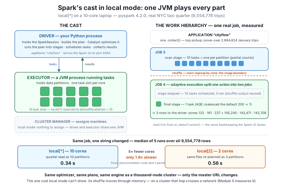
local[*] both share one JVM, with defaultParallelism resolving to 10 and no cluster manager needed. The hierarchy (right), from a real job: one .collect() over January's 2,964,624 trips became two jobs — a 10-task scan stage (one task per partition, cut at the shuffle), a skipped stage (10 scheduled, 0 ran — shuffle output reused), and a 1-task finish that adaptive execution coalesced from a default of 200. The measurement (bottom): the same quarter aggregation over 9,554,778 rows ran in a median 0.34 s on local[*] (10 partitions) and 0.56 s on local[2] — which re-planned the read as 3 partitions, because partitioning follows the cores available. 5x fewer cores, 1.6x the time: parallelism is real, sub-linear, and capped by the fixed costs cores can't touch. Only the master URL separates this from a cluster.One honest asterisk before this lesson closes, because this course promised to measure rather than romanticize.
When stage 4 shuffled its partial counts to stage 6, those bytes “moved” between tasks running as threads inside one JVM — the move was a memory hand-off measured in microseconds. On a real cluster, a shuffle means every executor writing sorted blocks to its local disk and every other executor pulling its share over the network, and that traffic is routinely the most expensive line item in a distributed job — the thing whole chapters of Spark tuning lore exist to minimize. Local mode runs the genuine shuffle machinery (the sort, the blocks, the bookkeeping — you saw its stage boundary in the tracker), but the genuine shuffle cost has no network to be paid on. So hold both truths: every plan, partition count, stage boundary, and task you inspect locally is real Spark behaviour that transfers to a cluster unchanged — and the one number that does not transfer is how much moving data between stages hurts. Module 5 takes exactly that on: it will make shuffle cost visible on this same laptop, measure it, and teach you to design jobs that move less.
The measuring is done, so end the application the way every Spark script should — explicitly:
spark.stop()
print("application over -- the UI on port 4040 went down with it")
application over -- the UI on port 4040 went down with itExercise 1 — Dial the cores and map the chain. The lesson measured local[*] (10 cores) and local[2]. Fill in the curve: run the same busiest_hours job under local[1], local[2], local[4], and local[*], and for each record defaultParallelism, the quarter’s partition count, and the median of five timed runs. Present the four rows as a table and answer two questions: is the partition count always equal to defaultParallelism, and is the speedup from 1 → 10 cores anywhere near 10x?
Hint
Build the sessions sequentially — spark.stop() before each new builder, or getOrCreate() will hand you the previous session and every “configuration” after the first will silently measure the same engine (print sc.master each round to prove you dodged the trap). Warm up each session with one untimed run before the five you record. Expect the partition count to track parallelism loosely, not exactly — Spark aims partition sizes at the slots available, subject to file boundaries — and expect the 1 → 10 speedup to fall well short of 10x for the same reason the lesson’s 5x core cut only cost 1.6x: the fixed costs of planning, scheduling, and collecting don’t scale with cores, and on a 153 MB job they are a big slice of the total.
Exercise 2 — Predict the anatomy, then check it. Before running anything, write down predictions — jobs, stages, tasks per stage — for three actions against the January DataFrame: (a) jan.count(), (b) jan.filter(F.col("PULocationID") == 132).count(), and (c) jan.groupBy("payment_type").count().collect(). Then run each under its own setJobGroup tag and pull the real anatomy from sc.statusTracker(), as the lesson did. Score your three predictions and explain every miss.
Hint
Reason from the two rules: tasks per stage = partitions (10 for January), and stages split at shuffles. A filter transforms each partition independently — no shuffle — so (a) and (b) should look alike in structure. A groupBy must shuffle, so (c) should reproduce the lesson’s shape: a 10-task scan stage, then a tiny reduce stage. Don’t be alarmed if AQE turns one action into two jobs or marks a stage skipped — the lesson hit both — and note that count() on a Parquet file can be suspiciously fast for a reason worth investigating: the file’s footer already knows the row count per row group.
Exercise 3 — Spend ten minutes inside the UI. Wrap the quarter aggregation in a loop of 20 runs so the application stays busy, open the address from sc.uiWebUrl, and go find four specific things: (1) your anatomy-style job group description in the Jobs list; (2) a skipped stage, rendered grey; (3) the task timeline for a 10-task scan stage — look at whether all ten tasks start together and which finishes last; (4) in the Environment tab, the values of spark.master and spark.sql.shuffle.partitions. Write one sentence per finding, and one more: which task in the timeline was the straggler, and by how much?
Hint
Keep the script alive or the UI vanishes with the session — either browse while the loop runs or park input("press Enter to stop") before spark.stop(). In the Jobs page, click a job, then a stage, then expand “Event Timeline.” The straggler question is not busywork: a stage finishes when its last task does, so one slow task holds every core hostage — that observation becomes the skew problem later in the course. If port 4040 shows a different application than you expect, you have two sessions alive and the trap from this lesson is already mid-bite.
Spark’s architecture is a cast of three: the driver runs your Python, holds the SparkSession, optimizes plans, and schedules work; executors hold partitions and run tasks; a cluster manager leases machines — a role that collapses in local mode, where driver and executors share one JVM and local[*] resolved to defaultParallelism of 10 on this machine. Work divides as application → job → stage → task: actions trigger jobs, shuffles cut stages, and each stage runs one task per partition — a rule verified live when January’s 48 MB file read as 10 partitions and its zone aggregation scheduled a 10-task scan stage. The full anatomy from the status tracker held two honest surprises: adaptive execution split one .collect() into two jobs, marked a 10-task repeat stage skipped (0 ran — shuffle output reused), and coalesced the reduce stage from a default of 200 tasks to 1. Every answer cross-checked against Course 1’s verified ground truth: 2,964,624 January rows, JFK’s 145,240 pickups, the quarter’s 9,554,778. The getOrCreate() trap is real and silent — with a session alive, a builder asking for local[2] got local[*] back, the identical object — so: one session at a time, stop() before rebuilding. Done right, the master string is a measured dial, and an honest one: the same quarter aggregation took a median 0.34 s on local[*] and 0.56 s on local[2] — only 1.6x slower on 5x fewer cores, because a 153 MB job is dominated by fixed planning-and-scheduling costs that cores can’t touch — and local[2] also re-planned the read from 10 partitions to 3, because partitioning follows the cores available. And one caveat holds the whole picture honest: local mode’s shuffle moves through memory, so the network cost that dominates real clusters is the one number a laptop cannot show — Module 5’s job.
local[*], local[N]) — the real engine with executor threads standing in for a cluster: same optimizer, plans, shuffle machinery, and UI. defaultParallelism follows the core count, and partition sizing follows it — local[2] read the same quarter as 3 partitions, not 10.getOrCreate() — returns any live session unmodified, silently ignoring the builder’s master and app name (only runtime SQL configs apply). One session at a time; stop() before reconfiguring; verify with sc.master or the UI’s Environment tab.CityFlow’s team is about to spend an entire course issuing commands to this engine, and the difference between using Spark and understanding it is exactly the ability this lesson practiced: predicting the machinery before it moves. When a query is slow, the answer is written in this lesson’s vocabulary — which job, which stage, how many tasks, and was the stage boundary a shuffle you could have avoided. When a benchmark makes no sense, the first suspect is now obvious: is the session you’re measuring the session you configured, or did getOrCreate() keep the old one alive? When Module 5 makes shuffles expensive on purpose, you already know where stages split and why. And the local-mode argument is the quiet confidence under all of it: because the laptop runs the genuine engine, every partition count, stage boundary, and plan you inspect this course is cluster truth, not classroom truth. The habits transfer with the code — one string, local[*] to a cluster URL, and the mental model you built against ten cores starts predicting the behaviour of a thousand.
You now know the cast, and you have already met the object that hires it: that SparkSession.builder block at the top of every script. Lesson 3, Your First SparkSession, slows down on it properly — which builder configs actually matter on a laptop and which are cluster cargo-cult, how to read the real quarter as one DataFrame instead of three files, and what Spark’s laziness means for the first honest queries CityFlow runs on the new engine: schema, counts, filters, and projections over all 9,554,778 trips. It also walks straight at the sharpest edge a PySpark beginner meets: toPandas(), the innocent-looking method that asks the driver to materialize an entire distributed DataFrame in one Python process — the same memory wall Course 1 spent a module dismantling, rebuilt with a single line. You’ll measure exactly when collecting to the driver is fine, when it is fatal, and how to tell before you run it. Bring the vocabulary from this lesson; every query from here on is jobs, stages, and tasks.
Keep DATATWEETS free. Help fund practical data, AI, and engineering lessons for learners worldwide.
