Title here
Summary here
Lesson 1 measured the ceiling of one machine, and Lesson 2 introduced the engine built past it — the driver that plans, the executors that execute — and proved that local mode runs the genuine article on a laptop. Both lessons handed you a running session and asked you to inspect it. That was deliberate sequencing, and it is now over: a data engineer who cannot stand Spark up from a blank terminal does not really have Spark, they have a notebook someone else configured. This lesson builds everything from scratch — the installation (both halves of it, because pip install pyspark is only one), the builder pattern config by config, and the first honest workload: CityFlow’s full quarter, all three monthly files, in a single read.
The workload is the point. Course 1 spent eight modules on this exact quarter and left behind ground truth verified to the cent — 9,554,778 trips across January, February, and March 2024, with known per-month counts and known busiest zones. So every number Spark produces today can be checked against numbers CityFlow already trusts, and every one will match to the row. Along the way you will see the two behaviours that most surprise pandas people on day one: a read of 160.4 MB that returns in 59 ms because it read nothing yet, and a toPandas() call on a single month that does not return at all — it kills the JVM with java.lang.OutOfMemoryError and takes the session down with it. We ran it so you don’t have to. Both behaviours come from the same architecture you met in Lesson 2, and both will make you a more deliberate engineer.
By the end of this lesson, you will be able to:
UnsupportedClassVersionError an incompatible Java producesappName, master("local[*]"), and the console/logging configs each docount() does real workselect / filter / groupBy queries on 9,554,778 real trips and cross-check the answers against Course 1’s verified ground truthtoPandas(), and explain exactly how the naive version diesYou’ll need pyspark and a JDK (17 or 21); pandas comes along for the final step. Let’s build the session.
The Python half is as ordinary as it looks:
python -m pip install pysparkThat installs PySpark — 4.2.0 at the time of writing — and you might reasonably believe you are done. You are not, and the reason is worth understanding rather than memorizing. Spark is not a Python program. The engine — optimizer, scheduler, memory management, the executors themselves — is written in Scala and runs on the JVM, the Java Virtual Machine. What pip installed is the Python interface: when you call spark.read.parquet(...), PySpark relays the call to a JVM process that does the actual work. No JVM, no Spark. And not just any JVM: Spark 4 requires Java 17 or 21.
That requirement fails in a specific, recognizable way, and you should see the failure before you see the fix, because you will meet it again — on a colleague’s machine, in a CI job, on a fresh laptop. Here is what happened on this machine when Spark 4 was pointed at an old JDK 11 (output wrapped for readability, middle trimmed):
Error: LinkageError occurred while loading main class org.apache.spark.launcher.Main
	java.lang.UnsupportedClassVersionError: org/apache/spark/launcher/Main has been
	compiled by a more recent version of the Java Runtime (class file version 61.0),
	this version of the Java Runtime only recognizes class file versions up to 55.0
...
pyspark.errors.exceptions.base.PySparkRuntimeError: [JAVA_GATEWAY_EXITED] Java gateway
process exited before sending its port number.
Read it from the bottom up, the way you will encounter it: the Python-side error says the “Java gateway process exited before sending its port number,” which sounds mysterious and tells you almost nothing except that the JVM died at birth. The real diagnosis is at the top: UnsupportedClassVersionError. Java class files carry a version number, and the decoder ring is that class file version 61.0 means “compiled for Java 17” while 55.0 means “this runtime is Java 11.” Spark’s launcher was compiled for a newer Java than the one that tried to load it. Whenever you see JAVA_GATEWAY_EXITED, scroll up and look for the class-file version line before you debug anything else.
The fix is to install a supported JDK and point the JAVA_HOME environment variable at it, in your shell — not in your Python code:
# macOS (Homebrew)
brew install openjdk@21
export JAVA_HOME="$(/usr/libexec/java_home -v 21)"

# Debian/Ubuntu
sudo apt install openjdk-21-jdk
export JAVA_HOME=/usr/lib/jvm/java-21-openjdk-amd64
JAVA_HOME is how PySpark’s launcher finds the JVM it should start. With it pointing at JDK 21, the same import that died above comes up cleanly — as you are about to see.
Set JAVA_HOME in your shell profile, never in your code
The export JAVA_HOME=... line belongs in ~/.zshrc or ~/.bashrc, so every terminal — and every scheduled job that inherits your environment — gets it for free. What it must never be is a hardcoded path inside your Python scripts: os.environ["JAVA_HOME"] = "/opt/homebrew/..." welds your laptop’s directory layout into code that will run on other machines, and it fails in the worst way — silently working for you and mysteriously breaking for everyone else. Environment configuration lives in the environment. Code that needs Java assumes Java is findable, and the shell makes it so.
With both halves installed, this is the whole ceremony — and every line of it earns its place:
import warnings
warnings.filterwarnings("ignore")
import time

from pyspark.sql import SparkSession

t0 = time.perf_counter()
spark = (SparkSession.builder
         .appName("cityflow")
         .master("local[*]")
         .config("spark.ui.showConsoleProgress", "false")
         .getOrCreate())
spark.sparkContext.setLogLevel("ERROR")
startup_secs = time.perf_counter() - t0

print("Spark version       :", spark.version)
print("master              :", spark.sparkContext.master)
print("default parallelism :", spark.sparkContext.defaultParallelism)
print("web UI              :", spark.sparkContext.uiWebUrl)
print(f"time to first session: {startup_secs:.1f} s")
Spark version : 4.2.0
master : local[*]
default parallelism : 10
web UI : http://localhost:4040
time to first session: 5.7 sTake the builder apart, because each call answers a different question:
SparkSession.builder — the entry point. A SparkSession is your handle on the whole engine: it owns the connection to the JVM, the SQL optimizer, and every DataFrame you create. One session per application is the rule, and the builder pattern — chain configuration calls, finish with getOrCreate() — is how you construct it..appName("cityflow") — a label, nothing more, but a label that follows the application into the web UI and the logs. When three jobs share a machine, the one named cityflow is findable and the one named pyspark-shell is not..master("local[*]") — the address of the cluster, and the most consequential line here. local[*] says: no cluster — run executors as threads inside this one JVM, one task slot per CPU core. That is where default parallelism : 10 comes from — this machine has 10 cores, so local[*] provisioned 10 slots. Lesson 2 dissected this mapping and measured local[2] against it; here it simply means every query below runs on all 10 cores with no further effort from us..config("spark.ui.showConsoleProgress", "false") — by default Spark draws animated progress bars in the terminal for every running stage. In an interactive shell they’re charming; in a script whose output you want to read or log, they interleave with your prints and make a mess. Off..getOrCreate() — creates the session, or hands you the existing one if this process already has one. The “or” hides a trap Lesson 2 demonstrated for real: if a session already exists, your configs are silently ignored. In a fresh script, it simply creates.setLogLevel("ERROR") — Spark ships chatty. At the default level, every job prints scheduler internals you don’t need while learning; at ERROR, Spark speaks only when something is genuinely wrong. (This one is a method call after creation, not a builder config, because it adjusts the live JVM’s logging.)Two honest notes on the printed facts. First, 5.7 s to a working session — that is real, it is mostly JVM startup, and it is the overhead half of this module’s argument: pandas needs no such runway, and Lesson 4 will weigh that cost properly. Second, the web UI: the printed address uses this machine’s network hostname, but http://localhost:4040 in a browser gets you the same place — a live dashboard of every job, stage, and task the session runs. Lesson 2 toured it; keep a tab open as you work through this lesson and you’ll see each query below appear as a job the moment it runs. (If port 4040 is taken — say, by a second Spark session — Spark quietly takes 4041 instead; the printed uiWebUrl always tells the truth.)
One thing you did not see: without the warnings.filterwarnings("ignore") at the top, pyspark 4.2 greets a machine with pandas 3.x installed with a FutureWarning: “PySpark does not yet fully support pandas >= 3.0.0. Some features may not work correctly.” We’ll come back to what that means when we actually touch pandas at the end of the lesson — for now it’s informational noise, which is why the filter is first.
The session is up. Point it at January — the same file Course 1 opened a hundred times — and time both the read and the count:
t0 = time.perf_counter()
jan = spark.read.parquet("yellow_tripdata_2024-01.parquet")
read_secs = time.perf_counter() - t0
print(f"read returned a {type(jan).__name__} in {read_secs:.2f} s")

t0 = time.perf_counter()
jan_rows = jan.count()
count_secs = time.perf_counter() - t0
print(f"count() returned {jan_rows:,} in {count_secs:.2f} s")
read returned a DataFrame in 1.72 s
count() returned 2,964,624 in 1.06 sThe count is instantly familiar — 2,964,624 is January’s row count, the same number Course 1’s chunked pandas pipeline established and re-verified for eight modules. Two engines, two languages, one answer. That agreement is the spine of this whole course: every Spark result gets checked against ground truth CityFlow already trusts.
The timings deserve a pandas-user’s double take. pd.read_parquet on this file materializes the month — by the time it returns, roughly 420 MB of DataFrame exists in RAM. Spark’s read.parquet returned in 1.72 s having materialized nothing. It opened the file’s footer, read the schema and row-group metadata, and gave you a DataFrame that is best understood as a description of data — which columns, which files — rather than the data itself. Even that 1.72 s overstates the file’s share: most of it is first-touch warmup (the JVM loading its I/O machinery), as the next section will prove by reading three times as much data in a thirtieth of the time. The count(), by contrast, is an action — it forced Spark to actually scan the file, and the scan is where the 1.06 s went.
That split — transformations describe, actions execute — is lazy evaluation, and it is one of the deepest differences between Spark and pandas. Module 2 owns that topic properly, including the query plans that make laziness an optimization superpower rather than a quirk. For today, one honest observation is enough: when a Spark line returns instantly, that is not speed — it’s deferral. Time the action, not the read.
You just read a file without declaring a single column type. Ask the DataFrame what it found:
jan.printSchema()root
|-- VendorID: integer (nullable = true)
|-- tpep_pickup_datetime: timestamp_ntz (nullable = true)
|-- tpep_dropoff_datetime: timestamp_ntz (nullable = true)
|-- passenger_count: long (nullable = true)
|-- trip_distance: double (nullable = true)
|-- RatecodeID: long (nullable = true)
|-- store_and_fwd_flag: string (nullable = true)
|-- PULocationID: integer (nullable = true)
|-- DOLocationID: integer (nullable = true)
|-- payment_type: long (nullable = true)
|-- fare_amount: double (nullable = true)
|-- extra: double (nullable = true)
|-- mta_tax: double (nullable = true)
|-- tip_amount: double (nullable = true)
|-- tolls_amount: double (nullable = true)
|-- improvement_surcharge: double (nullable = true)
|-- total_amount: double (nullable = true)
|-- congestion_surcharge: double (nullable = true)
|-- Airport_fee: double (nullable = true)Nineteen columns, correctly typed, for free — because Parquet embeds its schema in the file footer, and “inferring” it costs a metadata read, not a data scan. This is the same property Course 1 leaned on when it loaded only the columns it needed; Spark exploits it identically.
One type is worth a hard look: the timestamps read as timestamp_ntz — no time zone. That is Spark’s name for exactly what pandas called datetime64[us] on these same files: a wall-clock instant with no zone attached, stored in the Parquet file as microseconds. Same bytes, same semantics, two vocabularies. And it should trigger a Course 1 reflex: these are the columns where the microseconds-vs-nanoseconds unit trap lived — integer representations of these timestamps are microseconds, pd.Timestamp.value is nanoseconds, and mixing them matches zero rows without an error. Spark won’t make that particular mistake for you, but the moment you round-trip timestamps between Spark and pandas (as we will, shortly), you are back in unit-discipline territory. Know your resolution.
The remaining types are direct translations of what Course 1 profiled — PULocationID an integer, the money columns double, store_and_fwd_flag a string — and yes, a double for money will eventually need the same care it needed in pandas. Later modules take that up.
Here is where Spark’s file handling starts to feel like the tool CityFlow was promised. spark.read.parquet takes multiple paths — no loop, no pd.concat, no manual bookkeeping:
months = [
    "yellow_tripdata_2024-01.parquet",
    "yellow_tripdata_2024-02.parquet",
    "yellow_tripdata_2024-03.parquet",
]

t0 = time.perf_counter()
quarter = spark.read.parquet(*months)
read_secs = time.perf_counter() - t0
print(f"read of all three files returned in {read_secs * 1000:.0f} ms")

t0 = time.perf_counter()
for path in months:
    print(f"  {path}  {spark.read.parquet(path).count():>10,}")
total = quarter.count()
count_secs = time.perf_counter() - t0
print(f"  quarter total                       {total:>10,}")
print(f"(all four counts in {count_secs:.2f} s)")
read of all three files returned in 59 ms
yellow_tripdata_2024-01.parquet 2,964,624
yellow_tripdata_2024-02.parquet 3,007,526
yellow_tripdata_2024-03.parquet 3,582,628
quarter total 9,554,778
(all four counts in 0.48 s)Every number on that scoreboard is a handshake with Course 1. 2,964,624 • 3,007,526 • 3,582,628 — total 9,554,778: exactly the per-month and quarter counts the chunked pandas pipeline established, the numbers CityFlow’s whole reporting stack was verified against. Spark read the same bytes and reached the same truth, first try.
And now the laziness claim from the last section has proof. Reading all three files — 160.4 MB on disk — returned in 59 ms. Nobody reads 160 MB in 59 ms from a laptop’s SSD and parses it into 9.5 million rows; what returned was a plan. The earlier 1.72 s read really was warmup, just as promised. Meanwhile all four count() jobs — three per-file scans plus the full quarter — finished in 0.48 s combined, because a warmed-up engine with 10 task slots makes short work of counting Parquet. For comparison, Course 1’s first full-quarter row count required either 1.3 GB of materialized DataFrame or a deliberately engineered chunked loop. Spark’s version is one line, and the memory never moves.
The quarter DataFrame now covers the whole three months as a single logical table — no concatenation step, no seams. Every query from here on runs against all 9,554,778 rows.
The DataFrame API will feel familiar and slightly foreign at once — pandas taught you the vocabulary, Spark makes you say it more explicitly. Three verbs cover today: select picks columns, filter picks rows, show prints a sample. Ask for CityFlow’s favourite subject — JFK Airport pickups, zone 132:
from pyspark.sql import functions as F

jfk = (quarter
       .select("tpep_pickup_datetime", "PULocationID", "DOLocationID",
               "trip_distance", "total_amount")
       .filter(F.col("PULocationID") == 132))
jfk.show(5)
print(f"JFK pickups in the three files: {jfk.count():,}")
+--------------------+------------+------------+-------------+------------+
|tpep_pickup_datetime|PULocationID|DOLocationID|trip_distance|total_amount|
+--------------------+------------+------------+-------------+------------+
| 2024-01-01 00:50:09| 132| 216| 5.0| 25.45|
| 2024-01-01 00:46:16| 132| 239| 20.85| 82.69|
| 2024-01-01 00:50:28| 132| 26| 20.34| 86.25|
| 2024-01-01 00:06:29| 132| 170| 16.4| 82.69|
| 2024-01-01 00:55:31| 132| 213| 18.42| 79.29|
+--------------------+------------+------------+-------------+------------+
only showing top 5 rows
JFK pickups in the three files: 429,746The rows look right — New Year’s minutes after midnight, 16-to-20-mile airport runs, $80 totals. F.col("PULocationID") == 132 builds a column expression (that’s why the functions import matters — comparisons happen in the JVM, not in Python), select and filter are both lazy transformations, and only show and count did work.
But check the count against ground truth and something is off by one. Course 1’s quarter report says JFK had 429,745 pickups. Spark says 429,746. Who’s wrong?
Neither — and the discrepancy is a data-quality lesson wearing a very small disguise. Course 1’s report was built on a window: pickups from January 1 up to but not including April 1, with stray-timestamp rows quarantined — and it found 21 such strays, rows sitting in these files with pickup times like 2002 and 2009. Our jfk count has no window; it counts every row in the three files. One of those 21 strays is evidently a JFK pickup. Apply Course 1’s window and the number snaps into place:
in_window = jfk.filter(
    (F.col("tpep_pickup_datetime") >= "2024-01-01") &
    (F.col("tpep_pickup_datetime") < "2024-04-01")
)
print(f"JFK pickups inside the quarter window: {in_window.count():,}")
JFK pickups inside the quarter window: 429,745Exactly Course 1’s number. Hold onto the shape of what just happened: “the files” and “the quarter” are different populations, and a one-trip difference between two correct counts is the kind of thing that erodes a team’s trust in a new engine if nobody can explain it. Lesson 5’s guided project turns this into a formal quality gate — per-month stray counts and all. (Comparing a timestamp_ntz column against the string "2024-01-01" is safe, by the way: Spark parses the literal to a timestamp at plan time. The µs-vs-ns trap lives in integer round-trips, not string literals.)
Now the module’s flagship cross-check — the busiest January pickup zones, via the aggregation verb you already know:
(jan.groupBy("PULocationID")
    .count()
    .orderBy(F.col("count").desc())
    .show(3))
+------------+------+
|PULocationID| count|
+------------+------+
| 132|145240|
| 161|143471|
| 237|142708|
+------------+------+
only showing top 3 rows132 = 145,240 • 161 = 143,471 • 237 = 142,708. JFK first, then Midtown Center, then Upper East Side South — identical, trip for trip, to the January ranking Course 1 verified. The groupBy(...).count() chain reads almost like the pandas value_counts() it replaces, and under it, ten executor threads scanned January in parallel and merged their partial counts — the mechanics Lesson 2 dissected, now simply doing their job.
Every pandas user who meets Spark has the same thought within the hour: “fine, I’ll query in Spark, then toPandas() and work like a human being.” The instinct is half right, and the half that’s wrong is Course 1 Module 1’s memory wall wearing a new costume. toPandas() — like its lower-level sibling collect() — takes the distributed result and delivers all of it to the driver process, and the driver is one process on one machine. Executors can be many; the destination is one.
Here is the naive version, on just one month — not even the quarter. Do not run this line; we ran it for you, once, in a session exactly like this one:
# gate: skip
jan_pdf = jan.toPandas()   # January alone: 2,964,624 rows to one process
26/07/17 01:52:33 ERROR Executor: Exception in task 4.0 in stage 1.0 (TID 5)
java.lang.OutOfMemoryError: Java heap space
at java.base/java.lang.Integer.valueOf(Integer.java:1083)
at scala.runtime.BoxesRunTime.boxToInteger(BoxesRunTime.java:63)
...
py4j.protocol.Py4JJavaError: An error occurred while calling o42.getResult.
: org.apache.spark.SparkException: Exception thrown in awaitResult:
...
Caused by: org.apache.spark.SparkException: Job aborted due to stage failure: Task 4 in
stage 1.0 failed 1 times, most recent failure: Lost task 4.0 in stage 1.0 (TID 5)
(localhost executor driver): java.lang.OutOfMemoryError: Java heap space(Trimmed — the full traceback runs a couple of hundred lines. Every line shown is verbatim.)
That is a real, reproducible crash on a machine that Course 1 proved can hold this month in pandas comfortably. So why did Spark — the scaling engine — die on it? Look at the failure location: (localhost executor driver). In local mode, the executors are threads inside the driver’s JVM — one process, one heap — and that heap defaults to 1 GB (spark.driver.memory). January is roughly 420 MB as a pandas DataFrame, but to deliver it, the JVM must stage the collected rows in its own heap on the way to Python — and staging plus serialization plus the JVM’s own working set does not fit in 1 GB. The tasks themselves ran out of heap while packaging results. And the aftermath is worse than an exception: in our run, the JVM was wounded badly enough that the session did not survive — every subsequent Spark call failed with Job cancelled because SparkContext was shut down. One careless collect cost the whole application.
Could you raise spark.driver.memory to 4 GB and “fix” it? For one month, yes — and it would be exactly the mistake Course 1 Module 1 spent a lesson unteaching: buying headroom instead of changing shape. The quarter is 1,347 MB in pandas; a year is four times that; the pattern that needs the whole table on one process fails eventually, by construction, and the bigger heap just moves the funeral. We are not going to materialize the quarter to prove a wall Course 1 already measured — that money is spent.
The pattern that never hits the wall is the one Course 1’s streaming aggregations taught, translated to Spark: aggregate first, collect small. Do the 9.5-million-row work in Spark, where it parallelizes and never materializes; bring back only the answer, which is almost always tiny. The same window as Course 1’s report, the busiest zones of the whole quarter:
zone_counts = (quarter
               .filter((F.col("tpep_pickup_datetime") >= "2024-01-01") &
                       (F.col("tpep_pickup_datetime") < "2024-04-01"))
               .groupBy("PULocationID")
               .count()
               .orderBy(F.col("count").desc()))

t0 = time.perf_counter()
zones_pdf = zone_counts.toPandas()
agg_secs = time.perf_counter() - t0

print(f"aggregated 9,554,757 trips into {len(zones_pdf):,} rows "
      f"({zones_pdf.memory_usage(deep=True).sum() / 1024:.1f} KB) in {agg_secs:.2f} s")
print(zones_pdf.head(5).to_string(index=False))
aggregated 9,554,757 trips into 262 rows (3.2 KB) in 0.95 s
PULocationID count
161 453825
237 439138
132 429745
236 416508
162 336460Same verb, opposite outcome. This toPandas() moved 262 rows — 3.2 KB — across the JVM-to-Python boundary, in 0.95 s including the full 9,554,757-trip scan and aggregation. And the answer is Course 1’s quarter report to the row: Midtown Center 453,825, Upper East Side South 439,138, JFK 429,745, Upper East Side North 416,508, Midtown East 336,460. (Note the trip total: 9,554,757, not 9,554,778 — the window excluded the 21 strays, exactly as Course 1’s report did.) The DataFrame in zones_pdf is ordinary pandas; chart it, style it, hand it to the dashboard. That is the division of labour that carries you through the rest of this course: Spark owns the rows, pandas owns the result.
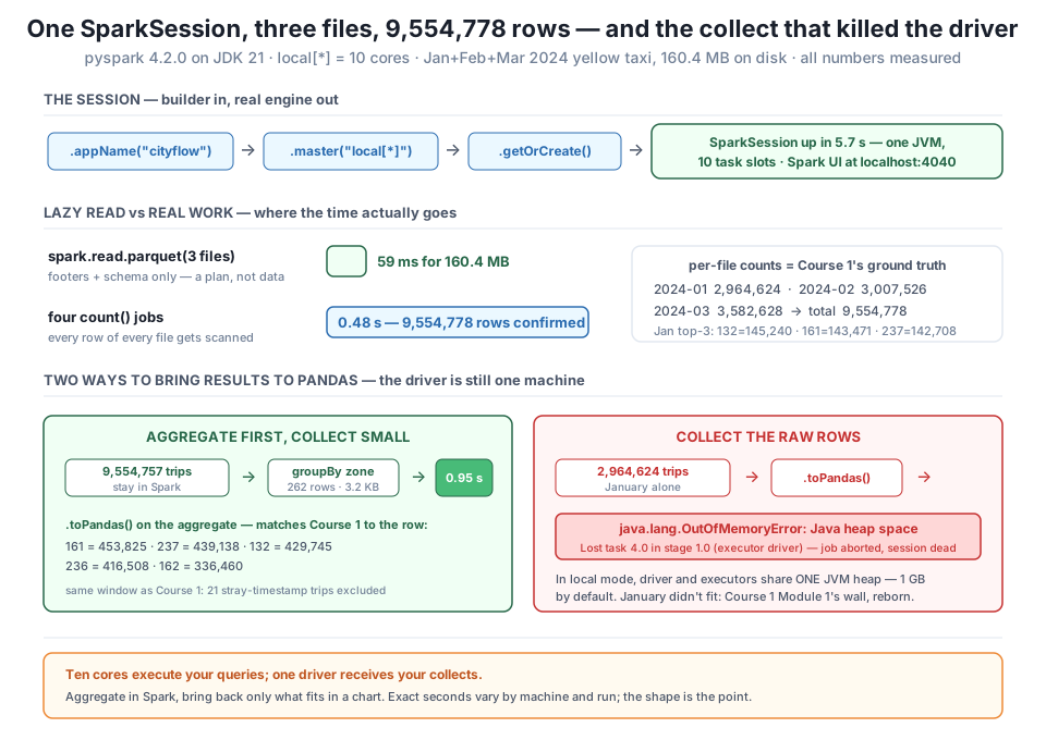
toPandas(), all measured on this machine. The builder produced a real engine in 5.7 s; reading all three files (160.4 MB) returned in 59 ms because a Spark read is a plan, not data, while four count() jobs scanned and confirmed 9,554,778 rows — Course 1's ground truth exactly — in 0.48 s. Bottom: aggregating 9,554,757 windowed trips to 262 rows (3.2 KB) before toPandas() took 0.95 s and reproduced Course 1's busiest-zone report to the row (161=453,825 · 237=439,138 · 132=429,745), while calling toPandas() on January's raw 2,964,624 rows killed the shared 1 GB local-mode heap with java.lang.OutOfMemoryError and took the whole session with it. Ten cores execute your queries; one driver receives your collects. Exact seconds vary by machine and run; the shape is the point.The pandas 3.0 warning, honestly
The FutureWarning we silenced at the top — “PySpark does not yet fully support pandas >= 3.0.0” — fires on import and again inside toPandas() on any machine running pandas 3.x, which by now is most of them. What it means in practice: the PySpark-to-pandas conversion path was written against pandas 2.x behaviour, and edge cases (mostly around dtype conversion) may differ until PySpark declares full support. Every result in this lesson — the 262-row aggregate, its dtypes, its values — came back correct under pandas 3.0.3, and we verified the values against Course 1 rather than trusting the conversion blindly. That is the general posture to take with any version-skew warning: don’t suppress it because it’s wrong; suppress it because it’s noise once you’ve verified the behaviour you depend on.
One habit before the exercises. A SparkSession is a JVM, ten scheduler threads, and a web server — real resources that outlive your last query until you release them. Scripts should end the way they began: deliberately.
spark.stop()
print("session stopped")
session stoppedIn a notebook you might keep one session alive all day (that’s what getOrCreate is for). In a pipeline script — and CityFlow’s Spark work is headed for scheduled scripts — stop() belongs at the end, always: it frees the port, flushes the logs, and makes the next run’s getOrCreate() genuinely create.
Exercise 1 — Spark reads CSVs too, but you pay for the schema. Parquet handed Spark 19 correct column types for free. CSVs don’t. Read Course 1’s zone dimension (taxi_zone_lookup.csv, 265 rows — grab it from /datasets/nyc-taxi/taxi_zone_lookup.csv if you don’t still have it) three ways: spark.read.csv(path) bare, then with header=True, then with header=True, inferSchema=True. After each, run printSchema() and show(3). Describe what each option bought you — and time the third read against the first: where does the extra time come from?
Hint
Bare csv() gives you columns named _c0, _c1, ... all typed string — Spark won’t even assume the first row is a header. header=True fixes the names but not the types; inferSchema=True fixes the types but costs an extra pass over the data, because unlike Parquet, a CSV carries no schema and Spark has to read the values to guess. On 265 rows the extra pass is invisible; on a 10 GB CSV it doubles your read. This is why data engineers treat Parquet as the default and CSV as an ingestion format to escape from — a theme Module 3 takes up properly.
Exercise 2 — February’s podium. January’s top three pickup zones were 132, 161, 237 — verified against Course 1 above. Run the same groupBy("PULocationID").count().orderBy(...) chain on February’s file alone. Does the same trio lead, in the same order? Then answer a question the lesson left implicit: does JFK’s share of pickups look different in February than January, and what might CityFlow’s analysts make of airport traffic as a fraction of the whole?
Hint
Read yellow_tripdata_2024-02.parquet into its own DataFrame and reuse the exact chain from the lesson — only the source changes. For the share question, you already know February’s total (3,007,526 from the scoreboard); divide the zone’s count by it. Compute January’s share the same way (145,240 of 2,964,624). Whether the ranking changes and whether the shares change are different questions — a zone can hold rank while quietly gaining or losing ground.
Exercise 3 — The dirtiest column, the safest collect. Course 1 flagged trip_distance as untrustworthy, with a maximum in the hundreds of thousands of miles. Confirm it in Spark: on the full quarter, compute the maximum trip_distance and the count of trips claiming more than 100 miles, and bring both numbers back to Python. Both answers together should cross the JVM boundary as a handful of values — make sure your code collects answers, never rows.
Hint
quarter.agg(F.max("trip_distance")) produces a one-row DataFrame — calling .first() on it is the aggregate-first pattern at its most extreme: 9,554,778 rows in, one value out. For the count, filter(F.col("trip_distance") > 100).count() returns a plain Python integer with no collect at all. If your Spark maximum matches Course 1’s ground truth (312,722 mi — a taxi ride to the Moon and partway back), you’ve cross-verified engines on the exact column where dirty data hides.
You built a SparkSession from a blank terminal and put it straight to work on CityFlow’s real quarter. Setup was two installs, not one — pip install pyspark plus a JDK 17/21, because Spark’s engine lives on the JVM — and you saw the exact failure an old Java produces (UnsupportedClassVersionError, class file version 61.0 vs 55.0, surfacing in Python as JAVA_GATEWAY_EXITED) and the fix (JAVA_HOME, set in the shell, never hardcoded). The builder pattern produced a working engine in 5.7 s: appName for identification, master("local[*]") for 10 task slots on 10 cores, progress bars and log noise turned down, the web UI live on port 4040. Then the measurements that define Spark’s character: reading all three monthly files — 160.4 MB — returned in 59 ms because a Spark read is a plan, not data, while four count() jobs did the real scanning in 0.48 s and matched Course 1’s ground truth to the row: 2,964,624 + 3,007,526 + 3,582,628 = 9,554,778. First queries cross-verified January’s podium exactly (132=145,240, 161=143,471, 237=142,708), and a one-trip discrepancy on JFK (429,746 in the files vs 429,745 in the window) turned out to be one of the quarter’s 21 known stray-timestamp rows — files and windows are different populations. Finally, the driver’s wall, measured: toPandas() on January alone killed local mode’s shared 1 GB heap with java.lang.OutOfMemoryError and took the session down, while aggregating first shrank 9,554,757 trips to 262 rows (3.2 KB) that crossed to pandas in 0.95 s — reproducing Course 1’s busiest-zone report exactly (161=453,825, 237=439,138, 132=429,745).
appName, master, config) into getOrCreate(). It owns the JVM connection, the optimizer, and every DataFrame; stop() releases it deliberately.pip install pyspark installs an interface, not an engine. Spark 4 needs Java 17/21, found via JAVA_HOME; the mismatch failure is UnsupportedClassVersionError (class file 61.0 = Java 17, 55.0 = Java 11) hiding under a JAVA_GATEWAY_EXITED.spark.read.parquet on 160.4 MB returned in 59 ms because it read footers and schema, not rows. count() and show() are actions that trigger real scans. An instant return is deferral, not speed — Module 2 turns this into an optimization story.toPandas()/collect() deliver everything to one process; on January’s raw rows that meant java.lang.OutOfMemoryError in a 1 GB shared heap and a dead session. Reduce in Spark, then move only the answer: 262 rows, 3.2 KB, 0.95 s.CityFlow now has a second engine producing the same certified numbers as the first, and the path there is the professional template: install honestly (both halves, knowing the failure modes), configure deliberately (every builder line answering a stated question), verify obsessively (never trust a new tool’s answer until it reproduces an old tool’s audited one). The two surprises this lesson measured are the two that actually bite teams adopting Spark. The instant read seduces people into believing Spark is infinitely fast until the first action reveals where the time really goes — and knowing that transformations describe, actions execute is the difference between reading a benchmark and being fooled by one. The toPandas() crash is the sharper edge: the whole point of Spark is escaping single-machine memory limits, and a single careless collect reinstates them — because the driver is, and always will be, one process on one machine. Course 1 taught CityFlow to stream aggregations precisely so the whole table never had to exist in one place; Spark automates that discipline across ten cores, but only for engineers who let the reduction happen inside the engine. Ten cores execute your queries; one driver receives your collects. Respect the asymmetry and the laptop behaves like a small cluster. Ignore it and the cluster behaves like a small laptop.
You now have a working session, verified data, and two honest surprises in your pocket. What you don’t yet have is a ruling on the question CityFlow’s engineers will actually ask: should we? January’s count took 1.06 s in Spark — but the session took 5.7 s to start, and Course 1’s tuned pandas could count that month faster than both. Lesson 4, When Spark Wins — and Loses, stages the fair fight: the same aggregations, pandas versus Spark, at one, two, and three months of data, with the JVM startup and planning overhead counted rather than hidden. The result is not a coronation — on small data, Spark loses, measurably, and a course that pretended otherwise would be selling you something. What the numbers show instead is where the gap narrows, where it flips, and why — the parallel scan that pays off only when there’s enough to scan, the materialization pandas can’t avoid and Spark never does. By the end of it you’ll have the judgment this module exists to build: not “Spark is faster,” but “here is the line, and here is which side of it CityFlow’s workload lives on.”
Keep DATATWEETS free. Help fund practical data, AI, and engineering lessons for learners worldwide.
