Title here
Summary here
Lesson 3 ended on a high: a real SparkSession over the full quarter, Jan’s JFK count landing on 145,240 exactly, and ten cores scanning Parquet in parallel. It would be easy to close the module there and let you walk away believing Spark is simply faster. It is not — not always, not here, and pretending otherwise would waste everything the previous course taught you about measuring before believing. CityFlow’s team is about to have the argument every data team has: someone wants to rewrite the monthly reports in Spark “because it scales,” someone else points out the pandas pipeline finishes before Spark’s JVM has even started, and both of them are right about something. This lesson replaces that argument with a matrix of measurements.
The move is one you have already made once. The previous course’s data structures module asked “should I build the index?” and answered it with a crossover: the index cost 237.7 ms to build and each scan cost 53.9 ms, so the index paid for itself after 4.4 questions. Spark is the same bargain at a much bigger scale. Its costs are mostly fixed — importing the library, starting a JVM, warming the code generator — while its benefit scales with the data: ten cores scanning in parallel, no full materialization, an optimizer doing the column pruning you’d otherwise do by hand. pandas is the opposite: near-zero fixed cost, but every marginal row is processed by one thread holding everything it loads. Two cost curves with different shapes should cross somewhere. This lesson times the same real aggregation — the zone-hour revenue report whose ground truth you already know to the cent — in three engines at three sizes, bills Spark’s startup separately and honestly, measures everyone’s memory in fresh processes, and reports where the crossover actually lands on this machine. Including the parts where Spark loses.
By the end of this lesson, you will be able to:
You’ll need pyspark, pandas, and pyarrow. Let’s find out who actually wins.
Write the two cost models down before touching a clock, because they tell you what to measure. pandas’ total time to answer a question over months of data is essentially all marginal — a tiny import, then one thread doing work proportional to the data:
Spark pays a fixed cost — JVM startup, session creation, first-job code generation — that pandas never pays, in exchange for a marginal cost that should be smaller: ten cores scan the quarter’s Parquet in parallel while pandas scans it on one. Set the two totals equal and the crossover falls out, exactly like the index crossover did: . And the formula carries a warning in its denominator — if is not actually smaller than , there is no crossover at all. Spark doesn’t win eventually by default; it wins eventually only against a rival with a steeper slope. That is a thing to measure, not assume, because we have two pandas rivals with very different slopes: the previous course’s naive load-everything baseline and its finished streaming pipeline.
Ground rules for the benchmark, stated up front so every number below is interpretable. Everything runs on the real quarter — the same three TLC Parquet files every lesson uses. Every engine computes the same report: filter pickups to the quarter window, group by zone and hour, count trips, and sum revenue — the aggregation whose ground truth the previous course pinned at 240,917 buckets, 9,554,757 trips, $256,692,373.14. The warm-up policy: every timed cell is one untimed warm-up call followed by the median of three timed calls, so the OS page cache and any lazy initialization are paid before the clock starts; Spark’s session is created once, outside all timings — but its creation cost is reported separately, because a reader running a script pays it every run, and hiding it would rig the contest.
import warnings
warnings.filterwarnings("ignore")
import os, sys, time, statistics, subprocess
import pandas as pd
import pyarrow.parquet as pq

FILES = ["yellow_tripdata_2024-01.parquet",
         "yellow_tripdata_2024-02.parquet",
         "yellow_tripdata_2024-03.parquet"]
COLS = ["tpep_pickup_datetime", "PULocationID", "total_amount"]
LO, HI = pd.Timestamp("2024-01-01"), pd.Timestamp("2024-04-01")

def bench(fn, *args):
    """One untimed warm-up call, then the median of three timed calls."""
    fn(*args)
    runs = []
    for _ in range(3):
        t0 = time.perf_counter()
        result = fn(*args)
        runs.append(time.perf_counter() - t0)
    return statistics.median(runs), result

wall, results = {}, {}
for f in FILES:
    print(f"{f}: {os.path.getsize(f)/1e6:5.1f} MB")
print(f"quarter on disk: {sum(os.path.getsize(f) for f in FILES)/1e6:.1f} MB")
yellow_tripdata_2024-01.parquet: 50.0 MB
yellow_tripdata_2024-02.parquet: 50.3 MB
yellow_tripdata_2024-03.parquet: 60.1 MB
quarter on disk: 160.4 MBOne honest disclosure before any contest: 160.4 MB is small data. It fits in RAM several times over, which means this benchmark sits deep in the region where Spark’s fixed costs matter most. That is deliberate — it’s the data you actually have, and the interesting question is precisely whether Spark can compete on a dataset this size, because the answer decides what CityFlow should use for the reports it runs today.
The naive baseline is the previous course’s starting point: read everything into one frame, then ask the question. The streaming contender is where that course ended — prune to the three needed columns, stream Parquet batches through a bounded buffer, aggregate each batch, merge the partial results. Same library, wildly different engineering. Bringing both matters, because “Spark vs pandas” is meaningless until you say which pandas.
def zone_hour_naive(files):
    """Course 1's starting point: load everything, then ask the question."""
    df = pd.concat([pd.read_parquet(f) for f in files], ignore_index=True)
    kept = df[(df["tpep_pickup_datetime"] >= LO) & (df["tpep_pickup_datetime"] < HI)]
    report = (kept.assign(hour=kept["tpep_pickup_datetime"].dt.floor("h"))
                  .groupby(["PULocationID", "hour"], observed=True)
                  .agg(trips=("total_amount", "size"),
                       revenue=("total_amount", "sum")))
    return len(report), int(report["trips"].sum()), round(float(report["revenue"].sum()), 2)

def zone_hour_streaming(files):
    """Course 1's finished pipeline: prune columns, stream batches, merge partials."""
    partials = []
    for f in files:
        for batch in pq.ParquetFile(f).iter_batches(batch_size=1_000_000, columns=COLS):
            chunk = batch.to_pandas()
            kept = chunk[(chunk["tpep_pickup_datetime"] >= LO) &
                         (chunk["tpep_pickup_datetime"] < HI)]
            partials.append(
                kept.assign(hour=kept["tpep_pickup_datetime"].dt.floor("h"))
                    .groupby(["PULocationID", "hour"], observed=True)
                    .agg(trips=("total_amount", "size"),
                         revenue=("total_amount", "sum")))
    report = pd.concat(partials).groupby(level=[0, 1]).sum()
    return len(report), int(report["trips"].sum()), round(float(report["revenue"].sum()), 2)

for name, fn in (("naive", zone_hour_naive), ("stream", zone_hour_streaming)):
    for k in (1, 2, 3):
        wall[(name, k)], results[(name, k)] = bench(fn, FILES[:k])

print(f"{'median wall seconds (warm)':<28}{'1 month':>10}{'2 months':>10}{'3 months':>10}")
print(f"{'pandas, one big frame':<28}" + "".join(f"{wall[('naive', k)]:>9.2f}s" for k in (1, 2, 3)))
print(f"{'pandas, streaming':<28}" + "".join(f"{wall[('stream', k)]:>9.2f}s" for k in (1, 2, 3)))
b, t, r = results[("stream", 3)]
print(f"streaming, 3 months -> {b:,} buckets, {t:,} trips, ${r:,.2f}")
median wall seconds (warm) 1 month 2 months 3 months
pandas, one big frame 0.26s 1.16s 2.99s
pandas, streaming 0.21s 0.38s 0.60s
streaming, 3 months -> 240,917 buckets, 9,554,757 trips, $256,692,373.14Two slopes, immediately visible. The big frame’s cost climbs steeply — 0.26 s to 2.99 s, about 1.37 s per additional month — because it reads and materializes all nineteen columns of every file before discarding sixteen of them. Streaming climbs gently — 0.21 s to 0.60 s, about 0.20 s per month — because it touches only the three columns the report needs and never holds more than a batch. That 5x gap at the 3-month mark is the previous course’s entire curriculum expressed as one ratio. And note the streaming result: exactly the ground-truth 240,917 / 9,554,757 / $256,692,373.14. The bar Spark has to clear is now set, and it is higher than “beat pandas” — it’s “beat the pandas of someone who finished the previous course.”
Now the challenger — and the first measurements that matter are the ones most benchmarks quietly delete. Everything Spark does before its first useful answer is fixed cost, so we time each piece: importing the library, building the session (which launches and connects to a JVM), and the first job ever run on that session, which pays one-time costs the second job won’t — Java’s JIT compilation warming up, Spark generating and compiling the bytecode for this query shape, the whole machinery going from cold to warm.
t0 = time.perf_counter()
from pyspark.sql import SparkSession
from pyspark.sql import functions as F
import_secs = time.perf_counter() - t0

t0 = time.perf_counter()
spark = (SparkSession.builder
         .appName("cityflow")
         .master("local[*]")
         .config("spark.ui.showConsoleProgress", "false")
         .getOrCreate())
spark.sparkContext.setLogLevel("ERROR")
session_secs = time.perf_counter() - t0

def zone_hour_spark(files):
    """The same aggregation, written against Spark's DataFrame API."""
    report = (spark.read.parquet(*files)
              .where((F.col("tpep_pickup_datetime") >= "2024-01-01") &
                     (F.col("tpep_pickup_datetime") < "2024-04-01"))
              .groupBy("PULocationID",
                       F.date_trunc("hour", "tpep_pickup_datetime").alias("hour"))
              .agg(F.count("*").alias("trips"),
                   F.sum("total_amount").alias("revenue")))
    rows = report.collect()
    return (len(rows), sum(r["trips"] for r in rows),
            round(sum(r["revenue"] for r in rows), 2))

t0 = time.perf_counter()
zone_hour_spark(FILES[:1])
first_job_secs = time.perf_counter() - t0

for k in (1, 2, 3):
    wall[("spark", k)], results[("spark", k)] = bench(zone_hour_spark, FILES[:k])

print(f"import pyspark               : {import_secs:5.2f} s")
print(f"create the SparkSession      : {session_secs:5.2f} s")
print(f"first job ever (1 month)     : {first_job_secs:5.2f} s")
print(f"same job again, warm         : {wall[('spark', 1)]:5.2f} s")
import pyspark : 0.07 s
create the SparkSession : 3.85 s
first job ever (1 month) : 4.83 s
same job again, warm : 0.74 sRead that last pair twice, because it is the lesson’s most important single contrast: the same one-month job cost 4.83 s the first time and 0.74 s the second. Nothing about the data changed — the 4.09-second difference is the engine warming up, paid once per session. Add it up and Spark’s fixed bill on this machine is 0.07 + 3.85 + 4.83 = 8.75 seconds before it has both delivered an answer and reached warm speed. Meanwhile pandas answered the same one-month question in 0.26 s with a fixed cost of roughly an import. This is not a flaw to engineer away; it is the price of admission for a JVM, a distributed scheduler, and a compiler that turns your query into custom bytecode — machinery whose value has to arrive later, in the slope.
Watch the warm-up happen at localhost:4040
While your session is alive, the Spark UI at http://localhost:4040 lists every job this block just ran. Open the first job and the repeat: same query, same data, wildly different wall time — and the UI shows you the stages and tasks behind both. Lesson 2’s job → stage → task hierarchy stops being a diagram the first time you see your own warm-up in it.
Everything measured under one policy, side by side — the session already open, so this is the best case for Spark, the view a notebook user gets after startup is a sunk cost.
labels = {"naive": "pandas, one big frame", "stream": "pandas, streaming",
          "spark": "Spark local[*], session open"}
print(f"{'median wall seconds (warm)':<30}{'1 month':>10}{'2 months':>10}{'3 months':>10}")
print("-" * 60)
for name in ("naive", "stream", "spark"):
    print(f"{labels[name]:<30}" + "".join(f"{wall[(name, k)]:>9.2f}s" for k in (1, 2, 3)))
print("-" * 60)
for k in (1, 2, 3):
    fastest = min(("naive", "stream", "spark"), key=lambda n: wall[(n, k)])
    print(f"{k} month{'s' if k > 1 else ' '}: fastest = {labels[fastest]}"
          f"  (Spark vs big frame {wall[('spark', k)]/wall[('naive', k)]:.2f}x,"
          f" vs streaming {wall[('spark', k)]/wall[('stream', k)]:.2f}x)")
median wall seconds (warm) 1 month 2 months 3 months
------------------------------------------------------------
pandas, one big frame 0.26s 1.16s 2.99s
pandas, streaming 0.21s 0.38s 0.60s
Spark local[*], session open 0.74s 1.11s 2.71s
------------------------------------------------------------
1 month : fastest = pandas, streaming (Spark vs big frame 2.83x, vs streaming 3.51x)
2 months: fastest = pandas, streaming (Spark vs big frame 0.96x, vs streaming 2.90x)
3 months: fastest = pandas, streaming (Spark vs big frame 0.90x, vs streaming 4.49x)There are two verdicts in that table, and they answer two different arguments.
Against the big frame, the crossover is real and it is close. At 1 month Spark loses clearly — 0.74 s against 0.26 s, 2.83x slower — because a 50 MB job cannot buy enough parallel work to cover even Spark’s warm per-job overhead. At 2 months the two are 1.11 s versus 1.16 s: treat that as a tie, because a 4% gap is inside the run-to-run jitter of both engines, and on re-runs of this benchmark the 2-month cell genuinely flips winners. By 3 months Spark is ahead for real, 2.71 s versus 2.99 s. Straight lines through the endpoints put the crossing just under two months — roughly 100 MB of this data on this machine. The shape is exactly the one the formula promised: Spark’s marginal cost per month ( 0.99 s) undercuts the big frame’s ( 1.37 s), so the lines had to cross, and the quarter you already have is just past the crossing.
Against streaming pandas, there is no crossover — and the formula says there never will be on this axis. Spark loses every cell, 2.9x to 4.5x, and the reason is in the slopes: streaming’s 0.20 s per month is five times shallower than Spark’s 0.99. When , has no positive solution; more months only widen the gap. A single thread that reads three columns and never materializes anything is astonishingly hard to beat on one machine at in-memory scale — ten cores don’t rescue Spark here, because Spark is doing fundamentally more per row (scheduling tasks, exchanging data between partitions for the shuffle, running a general-purpose engine) than a loop that was hand-shaped to this exact question. If this feels like it contradicts Spark’s reputation, hold that thought: the resolution is in the memory table below, and in what happens when the data stops fitting.
2.71 warm seconds for the quarter — but which parts of Spark cost what? The claim from Lesson 3 was that transformations are lazy and only actions pay. Let’s time the phases separately on one month: opening the files and reading the schema, building the entire query, and executing it.
t0 = time.perf_counter()
df = spark.read.parquet(FILES[0])
read_secs = time.perf_counter() - t0

t0 = time.perf_counter()
report = (df.where((F.col("tpep_pickup_datetime") >= "2024-01-01") &
                   (F.col("tpep_pickup_datetime") < "2024-04-01"))
            .groupBy("PULocationID",
                     F.date_trunc("hour", "tpep_pickup_datetime").alias("hour"))
            .agg(F.count("*").alias("trips"),
                 F.sum("total_amount").alias("revenue")))
build_secs = time.perf_counter() - t0

t0 = time.perf_counter()
rows = report.collect()
exec_secs = time.perf_counter() - t0

print(f"open files + read schema   : {read_secs*1000:6.1f} ms")
print(f"build the whole query      : {build_secs*1000:6.1f} ms   (lazy -- nothing ran)")
print(f"execute and collect        : {exec_secs:6.2f} s    ({len(rows):,} buckets)")
report.explain()
open files + read schema : 51.0 ms
build the whole query : 41.7 ms (lazy -- nothing ran)
execute and collect : 1.18 s (77,533 buckets)
== Physical Plan ==
AdaptiveSparkPlan isFinalPlan=true
+- == Final Plan ==
ResultQueryStage 1
+- *(2) HashAggregate(keys=[PULocationID#670, _groupingexpression#707], functions=[count(1), sum(total_amount#679)])
+- AQEShuffleRead coalesced
+- ShuffleQueryStage 0
+- Exchange hashpartitioning(PULocationID#670, _groupingexpression#707, 200), ...
+- *(1) HashAggregate(... functions=[partial_count(1), partial_sum(total_amount#679)])
+- *(1) Project [PULocationID#670, total_amount#679, ...]
+- *(1) Filter ((isnotnull(tpep_pickup_datetime#664) AND (tpep_pickup_datetime#664 >= 2024-01-01 00:00:00)) AND ...)
+- *(1) ColumnarToRow
+- FileScan parquet [tpep_pickup_datetime#664,PULocationID#670,total_amount#679] Batched: true, ...,
PushedFilters: [IsNotNull(tpep_pickup_datetime), GreaterThanOrEqual(tpep_pickup_datetime,2024-01-01T00:00), ...],
ReadSchema: struct<tpep_pickup_datetime:timestamp_ntz,PULocationID:int,total_amount:double>
+- == Initial Plan ==
...(The plan is shown trimmed: the very long FileScan line is elided with ..., and the Initial Plan — the same plan before adaptive execution refined it — is collapsed.)
First, the phase costs demolish a common intuition: planning is not where Spark’s time goes. Building the entire query — filter, group, two aggregations — took 41.7 ms, and that’s a one-shot measurement; execution took 1.18 s. (Notice that single execution ran slower than the 0.74 s median from the matrix — single timed runs bounce around, which is exactly why the matrix uses medians.) The overhead that makes Spark lose on small data is not “Spark spends ages planning”; it’s the fixed startup bill plus a per-job floor of task scheduling and shuffle machinery that even 50 MB of work can’t dilute.
Second, the plan itself repays the reading. The files hold nineteen columns; the ReadSchema at the bottom shows the scan reading exactly three — Spark’s optimizer pruned the columns automatically, which is precisely the optimization that separates our two pandas contenders, except nobody had to know to do it. One line up, PushedFilters shows the quarter-window filter pushed into the Parquet reader itself. And the Exchange hashpartitioning(..., 200) is the shuffle — rows with the same zone-hour key moving between partitions so they can be aggregated together, the genuinely distributed step that a groupby forces and that pandas simply doesn’t have (one thread, one memory space, nothing to exchange). You wrote naive-looking code and got expert-pandas treatment from a query optimizer; the toll for that service is the fixed cost you just measured. That trade — optimization you don’t have to think about, paid for in overhead — is Spark’s actual value proposition on one machine, and it becomes decisive in Module 2 when the queries stop being this simple.
Speed comparisons are meaningless between engines that disagree, so before any conclusions: do all three implementations return the same report at every size, and does it match what the previous course established?
GROUND_TRUTH = (240_917, 9_554_757, 256_692_373.14)
for k in (1, 2, 3):
    vals = {results[(name, k)] for name in ("naive", "stream", "spark")}
    b, t, r = results[("spark", k)]
    verdict = "all three engines agree" if len(vals) == 1 else f"DISAGREE: {vals}"
    print(f"{k} month{'s' if k > 1 else ' '}: {b:>7,} buckets  {t:>9,} trips  ${r:>14,.2f}  -> {verdict}")
print(f"Course 1 ground truth (3 months): {GROUND_TRUTH[0]:,} buckets  "
      f"{GROUND_TRUTH[1]:,} trips  ${GROUND_TRUTH[2]:,.2f}")
print(f"matches ground truth: {results[('spark', 3)] == GROUND_TRUTH}")
1 month : 77,533 buckets 2,964,609 trips $ 79,456,031.97 -> all three engines agree
2 months: 151,908 buckets 5,972,133 trips $159,529,610.19 -> all three engines agree
3 months: 240,917 buckets 9,554,757 trips $256,692,373.14 -> all three engines agree
Course 1 ground truth (3 months): 240,917 buckets 9,554,757 trips $256,692,373.14
matches ground truth: TrueNine cells, three engines, one answer per size — and the 3-month row is the previous course’s verified ground truth to the cent, from an engine that didn’t exist in that course. This is the habit this course keeps insisting on: a new engine earns trust by reproducing numbers you already trust, then gets to be compared on speed.
The matrix flattered Spark by keeping the session open. But CityFlow’s reports don’t run in a notebook with a warm engine idling — they run as python report.py on a schedule, and a script pays every fixed cost, every run. So the final measurement runs each contender in a fresh process, cold start to finished 3-month report, and measures peak memory at the same time — the previous course’s discipline of measuring memory in separate processes, because ru_maxrss is a high-water mark that never comes back down within a process. One wrinkle is new: Spark’s memory lives in two processes, the Python driver and the JVM it launched. ru_maxrss covers the driver; for the JVM we ask the session for the JVM’s own pid, then sample its resident size with ps from a background thread while the job runs.
SHARED = '''
import time, resource, sys
t0 = time.perf_counter()
SCALE = 1 if sys.platform == "darwin" else 1024   # ru_maxrss: bytes on macOS, KiB on Linux
FILES = ["yellow_tripdata_2024-01.parquet",
         "yellow_tripdata_2024-02.parquet",
         "yellow_tripdata_2024-03.parquet"]
'''

NAIVE_SCRIPT = SHARED + '''
import pandas as pd
df = pd.concat([pd.read_parquet(f) for f in FILES], ignore_index=True)
frame_mb = df.memory_usage(deep=True).sum() / 1e6
kept = df[(df["tpep_pickup_datetime"] >= pd.Timestamp("2024-01-01")) &
          (df["tpep_pickup_datetime"] < pd.Timestamp("2024-04-01"))]
report = (kept.assign(hour=kept["tpep_pickup_datetime"].dt.floor("h"))
              .groupby(["PULocationID", "hour"], observed=True)
              .agg(trips=("total_amount", "size"), revenue=("total_amount", "sum")))
wall = time.perf_counter() - t0
peak = resource.getrusage(resource.RUSAGE_SELF).ru_maxrss * SCALE / 1e6
print(f"pandas, one big frame : {wall:5.1f} s   peak RSS {peak:7,.0f} MB   ({len(report):,} buckets; frame alone {frame_mb:,.0f} MB)")
'''

STREAM_SCRIPT = SHARED + '''
import pandas as pd, pyarrow.parquet as pq
COLS = ["tpep_pickup_datetime", "PULocationID", "total_amount"]
partials = []
for f in FILES:
    for batch in pq.ParquetFile(f).iter_batches(batch_size=1_000_000, columns=COLS):
        chunk = batch.to_pandas()
        kept = chunk[(chunk["tpep_pickup_datetime"] >= pd.Timestamp("2024-01-01")) &
                     (chunk["tpep_pickup_datetime"] < pd.Timestamp("2024-04-01"))]
        partials.append(kept.assign(hour=kept["tpep_pickup_datetime"].dt.floor("h"))
                            .groupby(["PULocationID", "hour"], observed=True)
                            .agg(trips=("total_amount", "size"), revenue=("total_amount", "sum")))
report = pd.concat(partials).groupby(level=[0, 1]).sum()
wall = time.perf_counter() - t0
peak = resource.getrusage(resource.RUSAGE_SELF).ru_maxrss * SCALE / 1e6
print(f"pandas, streaming     : {wall:5.1f} s   peak RSS {peak:7,.0f} MB   ({len(report):,} buckets)")
'''

SPARK_SCRIPT = SHARED + '''
import subprocess, threading
from pyspark.sql import SparkSession
from pyspark.sql import functions as F
spark = (SparkSession.builder
         .appName("cityflow-memory")
         .master("local[*]")
         .config("spark.ui.showConsoleProgress", "false")
         .getOrCreate())
spark.sparkContext.setLogLevel("ERROR")

# Ask the JVM for its own pid, then sample its resident size while the job runs.
jvm_pid = int(spark._jvm.java.lang.ProcessHandle.current().pid())
jvm_peak, stop = [0], threading.Event()
def sample():
    while not stop.is_set():
        out = subprocess.run(["ps", "-o", "rss=", "-p", str(jvm_pid)],
                             capture_output=True, text=True).stdout.strip()
        if out:
            jvm_peak[0] = max(jvm_peak[0], int(out) * 1024)
        stop.wait(0.05)
sampler = threading.Thread(target=sample, daemon=True)
sampler.start()

rows = (spark.read.parquet(*FILES)
        .where((F.col("tpep_pickup_datetime") >= "2024-01-01") &
               (F.col("tpep_pickup_datetime") < "2024-04-01"))
        .groupBy("PULocationID", F.date_trunc("hour", "tpep_pickup_datetime").alias("hour"))
        .agg(F.count("*").alias("trips"), F.sum("total_amount").alias("revenue"))
        .collect())
stop.set(); sampler.join()
spark.stop()
wall = time.perf_counter() - t0
driver = resource.getrusage(resource.RUSAGE_SELF).ru_maxrss * SCALE / 1e6
jvm = jvm_peak[0] / 1e6
print(f"Spark local[*]        : {wall:5.1f} s   peak RSS {driver + jvm:7,.0f} MB   ({len(rows):,} buckets; driver {driver:,.0f} MB + JVM {jvm:,.0f} MB)")
'''

print("fresh process each, 3 months, cold start to finished report:")
for script in (NAIVE_SCRIPT, STREAM_SCRIPT, SPARK_SCRIPT):
    child = subprocess.run([sys.executable, "-c", script], capture_output=True, text=True)
    print(child.stdout.strip())
fresh process each, 3 months, cold start to finished report:
pandas, one big frame : 4.6 s peak RSS 3,811 MB (240,917 buckets; frame alone 1,347 MB)
pandas, streaming : 1.0 s peak RSS 461 MB (240,917 buckets)
Spark local[*] : 10.9 s peak RSS 1,323 MB (240,917 buckets; driver 246 MB + JVM 1,077 MB)The script view rewrites the time standings: Spark’s warm 3-month win evaporates, because the 8.75-second fixed bill is 80% of its 10.9-second run. As a scheduled script at this scale, Spark finishes dead last — 2.4x behind even the naive load, 10.9x behind streaming. If your job is “run one aggregation over 160 MB and exit,” Spark is unambiguously the wrong tool, and now you can say why with four measured numbers instead of a vibe.
The memory column is where Spark redeems itself — and it is genuinely interesting. The big frame’s peak hits 3,811 MB for a quarter that is 160 MB on disk: the frame itself materializes at 1,347 MB (the 8.4x inflation the previous course measured), and the concat, the filter’s copy, and the groupby machinery stack transient copies on top of that. Spark peaks at 1,323 MB — about a third of the naive load — without any manual chunking, because it never materializes the quarter; its executors stream column batches through partial aggregations, which is structurally the streaming pipeline’s trick, applied automatically. But the split matters: 246 MB of that is the Python driver, and 1,077 MB is the JVM, most of it engine rather than data — a JVM heap, code caches, and shuffle buffers that would look roughly this size for a job a tenth as big. Streaming pandas holds its Course-1 promise at 461 MB. So the memory ranking mirrors the time ranking’s logic: Spark’s memory, like its time, is fixed overhead plus a gentle slope — wasteful at small scale, and the reason it survives at scales where the big frame’s 24x-disk peak becomes a machine-killer.
Put the three views together — warm matrix, script view, memory — and CityFlow’s engine choice stops being an argument. The guide below is grounded in this lesson’s numbers; the figure carries all of them.
Data comfortably in memory, question asked once or twice (up to a few hundred MB here): plain pandas. A fresh process answered the 1-month question in well under a second; nothing with a JVM can compete below the crossover, and the crossover on this machine sits just under 100 MB against naive pandas — worse against good pandas.
Repeated batch reports on one machine, data up to a few GB: the previous course’s toolkit — pruned columns, streamed batches, bounded memory. This is the measured champion of this lesson: fastest at every size warm (0.60 s for the quarter), fastest cold (1.0 s), leanest (461 MB). Its marginal cost (0.20 s/month) is so low that Spark’s slope never catches it at in-memory scale. Treat “we should use Spark because it’s faster” as empirically false for this workload on this machine.
Approaching one machine’s edges — data several times RAM, queries too gnarly to hand-tune, or a team that shouldn’t have to: Spark in local mode starts earning its bill. It beat the naive load at 3 months warm (2.71 vs 2.99 s), held peak memory to a third of naive’s without anyone thinking about chunking, and — the part no pandas pipeline offers — its optimizer did the column pruning and filter pushdown for you. The moment the workload is ten joins written by five analysts instead of one hand-shaped groupby, “automatic” stops being a convenience and becomes the difference between the naive and expert columns of this lesson’s matrix.
Beyond one machine: no contest, because the alternatives simply end. Lesson 1 established the ceiling — one machine’s cores saturate, its disk has one throughput, its RAM has one limit, and streaming defers that limit but never removes it. Spark’s fixed cost buys the one thing no pandas variant has at any price: local[*] becomes a cluster URL and the same code runs on forty machines. Module 2 starts cashing that check.
One caution, and it is not fine print: the crossover you just measured belongs to this machine and this workload. Ten cores, a fast SSD, 160 MB of clean Parquet, one groupby — change any of these and the numbers move, sometimes a lot. A slower disk flatters Spark’s parallel reads; a shuffle-heavy join punishes single-threaded pandas far more than this aggregation did; a 4-core laptop halves Spark’s parallel benefit. What transfers is the shape: Spark = fixed cost + shallow slope, pandas = no fixed cost + steeper slope, crossover = if the denominator is positive. Measure once and the two slopes with three sizes — twenty minutes of work, as you just saw — and you have your machine’s version of this figure instead of a stranger’s.
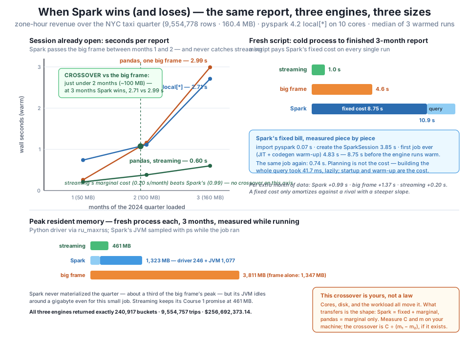
import 0.07 s + session 3.85 s + first-job warm-up 4.83 s = 8.75 s every run — 80% of Spark’s 10.9 s cold total — while the same job repeats warm in 0.74 s and building the whole query takes 41.7 ms. Bottom — memory: Spark peaks at 1,323 MB (246 driver + 1,077 JVM), a third of the big frame’s 3,811 MB, with no manual chunking; streaming holds 461 MB. All three engines agree to the cent: 240,917 buckets, 9,554,757 trips, $256,692,373.14. The digits are this machine’s; the shape — fixed cost amortized by a shallower slope, or not — is what transfers.Close the session — the last honest measurement is remembering the engine is still running until you stop it.
spark.stop()Why the 2-month cell is a coin flip
The matrix says Spark won the 2-month cell by 0.05 s. Re-run the benchmark and it will sometimes say the opposite — medians of three tame the jitter but don’t eliminate it, and a 4% gap is smaller than the jitter. The honest reading of any benchmark this close is “tie,” and the honest use of this lesson is the ratios and the slopes, not the second decimal. That is also why every timing section here states its policy (warm-up, medians, session outside the clock): a benchmark that doesn’t state its policy isn’t evidence, it’s an anecdote.
Exercise 1 — Find the floor. The matrix’s smallest cell was 2.96 million rows. Go far below the crossover: yellow_tripdata_sample.csv holds 200,000 trips. Time a per-zone revenue sum (groupby("PULocationID")["total_amount"].sum()) in pandas, then the same in Spark (spark.read.csv(..., header=True, inferSchema=True) and a groupBy) with a warmed session, using the lesson’s bench policy. Predict the ratio before you run it, then explain what Spark spends its extra time on when the data is this small.
Hint
Expect pandas to land around a quarter of a second and warm Spark around a second — a worse ratio than any Parquet cell in the matrix. Two effects stack: Spark’s per-job floor (task scheduling, a 200-partition shuffle for a job that fits in one hand) doesn’t shrink with the data, and inferSchema=True forces an extra pass over the CSV just to guess types. At 200k rows you are paying cluster overheads for a job a Counter could do.
Exercise 2 — Solve for the crossover you can’t see. Using the script-view numbers, compute each engine’s marginal cost per month from the warm matrix (), then solve for script-mode Spark against the big frame with s. You should get a crossover of roughly two years of data. Then write two sentences on why that crossover would never actually be reached by the big frame — check the memory column before you answer.
Hint
The slopes from this run: big frame ≈ 1.37 s/month, Spark ≈ 0.99, streaming ≈ 0.20. So months. But the big frame already peaked at 3,811 MB for 3 months — scale that linearly to 23 months and you need roughly 29 GB of RAM for a 1.2 GB-on-disk question. The big frame exits the race by running out of memory long before it loses on time — which is the real reason “when does Spark win?” is usually a memory question wearing a speed costume. Note there is no against streaming at all: its slope is below Spark’s, so only a workload that breaks streaming’s assumptions (shuffle-heavy joins, aggregation state that outgrows RAM, needing all cores) changes the verdict.
Exercise 3 — Turn the biggest visible knob. The physical plan showed Exchange hashpartitioning(..., 200): Spark shuffled our 240,917 aggregated rows into 200 partitions — a cluster default, absurd for one laptop. In a fresh session, time the 3-month report with the default, then set spark.conf.set("spark.sql.shuffle.partitions", "10") and time it again with the same bench policy. Report the speedup and explain why the default hurts more at small scale than large.
Hint
Expect a real but not miraculous win — on this machine the 3-month job dropped from about 2.1 s to about 1.6 s, roughly 25%. Each shuffle partition becomes a task with fixed scheduling cost; 200 tasks to aggregate 240,917 small rows is almost pure overhead, while 10 matches the core count. It doesn’t rescue the streaming comparison, because the scan — not the shuffle — dominates this job. Adaptive Query Execution (the AQEShuffleRead coalesced line in the plan) already merges some of the waste, which is why the win isn’t larger; Module 2 turns this knob with more context.
You measured the argument instead of having it. The frame first: pandas’ cost is nearly all marginal, Spark’s is a fixed bill plus a shallower slope, so the crossover — if it exists — sits at , the same arithmetic that priced the previous course’s index at 4.4 queries. Then the numbers, all from the real quarter and all agreeing to the cent (240,917 buckets, 9,554,757 trips, $256,692,373.14, three engines, every size). Warm, with the session cost sunk: Spark lost the 1-month cell 2.83x (0.74 s vs 0.26 s), tied the big frame at 2 months (1.11 vs 1.16 s — inside the jitter), and won at 3 months (2.71 vs 2.99 s), a measured crossover just under 2 months (≈100 MB) driven by the slopes: 0.99 s/month against 1.37. Against streaming pandas (0.21/0.38/0.60 s) Spark lost every cell by 2.9–4.5x, and the slopes say it always will at this scale — 0.20 s/month is below Spark’s 0.99, so no positive exists. Spark’s fixed bill, itemized: 0.07 s import + 3.85 s session + 4.83 s first-job warm-up = 8.75 s, against 41.7 ms to build the entire query — startup and warm-up are the cost, planning isn’t, and the plan repaid inspection anyway (automatic column pruning to a 3-column ReadSchema out of 19, filters pushed into the scan, the shuffle exposed). The script view: cold, Spark finished last at 10.9 s (80% of it the fixed bill) against 4.6 s naive and 1.0 s streaming — but peaked at 1,323 MB (246 driver + 1,077 JVM), a third of the big frame’s 3,811 MB, with no manual chunking, while streaming held 461 MB. Spark on one machine is exactly what its cost structure says: the wrong tool below the crossover, a memory-safe automatic optimizer near it, and the only tool whose code survives past the machine.
CityFlow’s monthly reports are 160 MB jobs that run on a schedule — and this lesson says, with numbers, that rewriting them in Spark today would make them ten times slower (10.9 s vs 1.0 s cold) while tripling their memory. That’s not an anti-Spark conclusion; it’s the reason the team can trust the pro-Spark conclusion coming. The same measurements show the naive path — the one most teams are actually on, because most code is written quickly by people mid-deadline — already loses to Spark at one quarter of data and dies of memory around two years’ worth, while Spark holds a third of the peak with an optimizer doing the pruning nobody remembered to do. The engineering skill is refusing to let either camp argue from reputation: you now itemize an engine’s fixed bill, fit two slopes with three sizes, check the denominator before promising a crossover, and verify both engines agree to the cent before comparing their clocks. Ten million trips fit on one machine; the next order of magnitude won’t, and when CityFlow crosses that line, the code you benchmarked today is the code that goes — unchanged — to the machines that can.
Module 1 has done its arguing: you know why one machine ends (Lesson 1), how Spark is shaped (Lesson 2), how to hold a session properly (Lesson 3), and now — measured, not asserted — where the engine wins and loses on the hardware in front of you. Lesson 5, Guided Project: The Quarter in Spark, turns all of it into CityFlow’s first shipped Spark artifact: one job that loads all three months, prints a unified schema, verifies every per-month count against the ground truth you’ve been cross-checking all module, flags the stray timestamps the previous course quarantined, ranks the busiest zones, and writes a one-page “state of the quarter” report a teammate could read without running anything. You’ll build it against acceptance criteria, the way real pipeline code gets built — and after this lesson, you’ll know exactly what that job’s 8.75-second opening silence is buying.
Keep DATATWEETS free. Help fund practical data, AI, and engineering lessons for learners worldwide.
