Title here
Summary here
This module has been an argument in four parts. Lesson 1 found the honest ceiling of one machine; Lesson 2 met the engine built past it and showed that local[*] runs the real thing; Lesson 3 started your first SparkSession and read the quarter; Lesson 4 measured, without flattery, where Spark loses to pandas and why. What’s still missing is the thing CityFlow actually pays for: an artifact. Not a notebook of experiments — a job. Something a teammate can run next Tuesday, on a machine you’ve never seen, and get the same page of numbers you got today.
That job is this project: a “State of the Quarter” report — CityFlow’s first production Spark script. It loads all three months of 2024 Q1 in one read, proves it got every row, surfaces the dirt this dataset is known to carry without deleting any of it, ranks the quarter’s busiest zones by their real names, and totals the revenue. And because the previous course already established every one of those numbers with pandas and pyarrow — down to the cent — this project has a property most first Spark jobs never get: a complete answer key. Course 1 says the quarter holds 9,554,778 trips, that 21 of them fall outside the quarter window, that Midtown Center leads with 453,825 pickups, and that the window’s revenue is exactly $256,692,373.14. If the new engine disagrees with any of that, the job — not the ground truth — is wrong. By the end of this page, a single script checks all of it, prints one page, and passes 12 of 12 cross-checks.
By the end of this project, you will be able to:
input_file_name() and reconcile per-month counts against known ground truthmain(), explicit cross-checks, and spark.stop() at the endYou’ll need pyspark (with the Java 17/21 runtime from the course setup page) — everything else is the Python standard library.
A guided project without acceptance criteria is just typing. Before any code, here is what “done” means for CityFlow’s first Spark artifact:
read.parquet call — not three DataFrames stitched together by hand.PULocationID and joined to real names from the zone lookup — and the top five must match Course 1’s ranking trip for trip.total_amount inside must print as $256,692,373.14.main() that creates its session, prints one report page with every check labelled, and calls spark.stop() — safe to re-run forever.The data is New York City’s public-domain Yellow Taxi trip records, published by the NYC Taxi & Limousine Commission on its Trip Record Data page — the same three months Course 1 processed, plus the zone lookup:
https://d37ci6vzurychx.cloudfront.net/trip-data/yellow_tripdata_2024-01.parquet (2,964,624 rows, 48 MB)https://d37ci6vzurychx.cloudfront.net/trip-data/yellow_tripdata_2024-02.parquet (3,007,526 rows, 48 MB)https://d37ci6vzurychx.cloudfront.net/trip-data/yellow_tripdata_2024-03.parquet (3,582,628 rows, 57 MB)https://datatweets.com/datasets/nyc-taxi/taxi_zone_lookup.csv (265 zones)A real pipeline downloads once and reads local copies afterwards, so every runnable block below uses the bare filenames:
# gate: skip
# Fetch once; every block afterwards reads the local cached copies by name.
import urllib.request
for m in ("01", "02", "03"):
    urllib.request.urlretrieve(
        f"https://d37ci6vzurychx.cloudfront.net/trip-data/yellow_tripdata_2024-{m}.parquet",
        f"yellow_tripdata_2024-{m}.parquet")
urllib.request.urlretrieve(
    "https://datatweets.com/datasets/nyc-taxi/taxi_zone_lookup.csv",
"taxi_zone_lookup.csv")A production job creates its SparkSession once, uses it for everything, and stops it on the way out. This is the same builder shape as Lesson 3 — local[*] for all ten cores, progress bars off so the output stays readable, log level at ERROR so warnings don’t bury results.
import warnings; warnings.filterwarnings("ignore")
import os
import time
from pyspark.sql import SparkSession
from pyspark.sql import functions as F

t0 = time.perf_counter()
spark = (SparkSession.builder
         .appName("cityflow-quarter")
         .master("local[*]")
         .config("spark.ui.showConsoleProgress", "false")
         .getOrCreate())
spark.sparkContext.setLogLevel("ERROR")
print(f"SparkSession up in {time.perf_counter() - t0:.1f} s "
      f"(Spark {spark.version}, master {spark.sparkContext.master})")
SparkSession up in 5.7 s (Spark 4.2.0, master local[*])There is Lesson 4’s tax, paid up front and in the open: 5.7 seconds before a single row moves. For the rest of this job it’s already spent — every step below runs against a warm engine, and the Spark UI is live at localhost:4040 if you want to watch the jobs land while the script runs.
Course 1 spent an entire module learning to process these three files one chunk at a time, because pandas would materialize them at 8.4x their disk size. Spark’s answer to the same problem is almost anticlimactic: pass all three paths to one read.parquet call and treat the result as a single table.
PATHS = [f"yellow_tripdata_2024-{m:02d}.parquet" for m in (1, 2, 3)]
on_disk = sum(os.path.getsize(p) for p in PATHS) / 1e6

t0 = time.perf_counter()
trips = spark.read.parquet(*PATHS)
t_read = time.perf_counter() - t0

t0 = time.perf_counter()
total = trips.count()
t_count = time.perf_counter() - t0

print(f"3 files, {on_disk:.1f} MB on disk")
print(f"read.parquet(...) returned in {t_read:.2f} s")
print(f"count() -> {total:,} rows in {t_count:.2f} s")
3 files, 160.4 MB on disk
read.parquet(...) returned in 1.91 s
count() -> 9,554,778 rows in 3.25 sThe total is 9,554,778 — criterion 2’s headline number, on the first try. But look at the two timings, because they are quietly strange. read.parquet “read” 160.4 MB across three files in 1.91 s — yet it read no trip data at all. It opened the file footers, checked that the three schemas agree, and handed back a plan. The count() that followed is the call that actually visited all ten million rows, across every row group in every file, on all ten cores. Hold on to that asymmetry — it is not an optimization detail, it is the design of the engine, and it’s exactly where Module 2 picks up.
Criterion 1 asks for one DataFrame with one schema. Verify it rather than assuming it — three files written months apart by someone else’s pipeline are three chances for a column to change type.
trips.printSchema()root
|-- VendorID: integer (nullable = true)
|-- tpep_pickup_datetime: timestamp_ntz (nullable = true)
|-- tpep_dropoff_datetime: timestamp_ntz (nullable = true)
|-- passenger_count: long (nullable = true)
|-- trip_distance: double (nullable = true)
|-- RatecodeID: long (nullable = true)
|-- store_and_fwd_flag: string (nullable = true)
|-- PULocationID: integer (nullable = true)
|-- DOLocationID: integer (nullable = true)
|-- payment_type: long (nullable = true)
|-- fare_amount: double (nullable = true)
|-- extra: double (nullable = true)
|-- mta_tax: double (nullable = true)
|-- tip_amount: double (nullable = true)
|-- tolls_amount: double (nullable = true)
|-- improvement_surcharge: double (nullable = true)
|-- total_amount: double (nullable = true)
|-- congestion_surcharge: double (nullable = true)
|-- Airport_fee: double (nullable = true)Nineteen columns, consistent across all three files. One type deserves a pause: the timestamps come back as timestamp_ntz — no time zone, exactly what the parquet files store (microsecond-precision wall-clock values). Course 1 had a whole trap around this column: mixing microsecond and nanosecond integer representations silently matched zero rows. In Spark you’ll compare it against plain strings like "2024-01-01" and the engine casts the literal to the column’s type for you — one entire class of unit bug retired by the type system.
The quarter total matching is necessary, not sufficient — two months could be swapped, or one file could hold another’s rows, and 9,554,778 would still print. Criterion 2 wants per-month counts, which poses a real question: after three files melt into one DataFrame, which row came from where?
Spark keeps the answer available: input_file_name() returns, for every row, the path of the file it was read from. One regex turns that into a source_month tag, and a groupBy turns the tag into the reconciliation table:
GROUND_ROWS = {"2024-01": 2_964_624, "2024-02": 3_007_526, "2024-03": 3_582_628}

tagged = trips.withColumn(
    "source_month",
    F.regexp_extract(F.input_file_name(), r"yellow_tripdata_(\d{4}-\d{2})", 1))

per_month = {r["source_month"]: r["n"]
             for r in tagged.groupBy("source_month").agg(F.count("*").alias("n")).collect()}
for m in sorted(per_month):
    status = "OK" if per_month[m] == GROUND_ROWS[m] else "MISMATCH"
    print(f"  {m}: {per_month[m]:>9,}   expected {GROUND_ROWS[m]:>9,}   {status}")
q_total = sum(per_month.values())
print(f"  quarter: {q_total:>9,}   expected 9,554,778   "
      f"{'OK' if q_total == 9_554_778 else 'MISMATCH'}")
2024-01: 2,964,624 expected 2,964,624 OK
2024-02: 3,007,526 expected 3,007,526 OK
2024-03: 3,582,628 expected 3,582,628 OK
quarter: 9,554,778 expected 9,554,778 OKFour checks, four OKs. This is the moment the new engine earns its first trust: a completely different runtime — JVM, distributed planner, parallel scan — agrees with Course 1’s pyarrow row counts exactly, month by month. Note the shape of the check, too: the expected values are written into the code and compared mechanically. A human eyeballing “yeah, that looks like about three million” is how a swapped file survives into production.
Course 1 established that every one of these files contains stray timestamps — pickups dated outside the month the file is named for: 18 in January, 15 in February, 23 in March, including relics from 2002 and 2009. A first-look job that doesn’t reproduce a known defect isn’t confirming the data is clean; it’s confirming the job can’t see.
The tagged frame makes the per-file check natural: derive each row’s expected month boundaries from its source_month, then count the rows that fall outside their own file’s month.
EXPECTED_STRAYS = {"2024-01": 18, "2024-02": 15, "2024-03": 23}

bounded = (tagged
           .withColumn("month_start",
                       F.to_timestamp(F.concat("source_month", F.lit("-01"))))
           .withColumn("month_end",
                       F.add_months("month_start", 1).cast("timestamp")))
stray = bounded.where((F.col("tpep_pickup_datetime") < F.col("month_start")) |
                      (F.col("tpep_pickup_datetime") >= F.col("month_end")))

for r in stray.groupBy("source_month").count().orderBy("source_month").collect():
    m, n = r["source_month"], r["count"]
    status = "OK" if n == EXPECTED_STRAYS[m] else "MISMATCH"
    print(f"  {m}: {n:>2} stray pickups   expected {EXPECTED_STRAYS[m]:>2}   {status}")

(stray.select("source_month", "tpep_pickup_datetime")
 .orderBy("tpep_pickup_datetime")
 .show(6, truncate=False))
2024-01: 18 stray pickups expected 18 OK
2024-02: 15 stray pickups expected 15 OK
2024-03: 23 stray pickups expected 23 OK
+------------+--------------------+
|source_month|tpep_pickup_datetime|
+------------+--------------------+
|2024-03 |2002-12-31 22:17:10 |
|2024-01 |2002-12-31 22:59:39 |
|2024-01 |2002-12-31 22:59:39 |
|2024-03 |2002-12-31 23:08:30 |
|2024-02 |2008-12-31 22:52:49 |
|2024-02 |2009-01-01 00:02:13 |
+------------+--------------------+
only showing top 6 rows18 / 15 / 23 — the dirt census matches Course 1 exactly, and the listing holds a small surprise the previous course never saw. Course 1’s deepest dive was January, whose oldest stamp is the famous 2002-12-31 22:59:39 (appearing twice — two different trips stamped with the same impossible second). But the quarter’s earliest pickup is 2002-12-31 22:17:10, and it lives in the March file. Every file in this feed carries its own decades-old relics; the defect is systemic to the TLC’s pipeline, not a one-off in one month. That’s a genuinely new finding, and it cost three lines of Spark.
Here’s a reconciliation that looks like a contradiction until you resolve it, and resolving it is worth a whole step. The per-file strays total . But Course 1’s quarter-level report quarantined only 21 rows. Both numbers are correct — they answer different questions.
LO, HI = "2024-01-01", "2024-04-01"
in_window = trips.where((F.col("tpep_pickup_datetime") >= LO) &
                        (F.col("tpep_pickup_datetime") < HI))

kept = in_window.count()
stray_total = stray.count()
spill = stray.where((F.col("tpep_pickup_datetime") >= LO) &
                    (F.col("tpep_pickup_datetime") < HI)).count()

print(f"per-month strays              : {stray_total}")
print(f"  still inside the quarter    : {spill}  (month-boundary spill)")
print(f"  outside the quarter entirely: {stray_total - spill}")
print(f"rows the quarter window keeps : {kept:,}   expected 9,554,757   "
      f"{'OK' if kept == 9_554_757 else 'MISMATCH'}")
print(f"rows the window quarantines   : {total - kept}   expected 21   "
      f"{'OK' if total - kept == 21 else 'MISMATCH'}")
per-month strays : 56
still inside the quarter : 35 (month-boundary spill)
outside the quarter entirely: 21
rows the quarter window keeps : 9,554,757 expected 9,554,757 OK
rows the window quarantines : 21 expected 21 OK35 of the 56 strays are month-boundary spill: a trip stamped 2024-02-01 00:00 sitting in the January file is wrong for its file but right for the quarter — a real fare that a report over Q1 must include. Only 21 rows — the 2002/2008/2009 relics, the late-December 2023 stamps, the few that leak past April 1st — fall outside the quarter entirely, and 9,554,757 kept / 21 quarantined matches Course 1’s zone-hour report to the row.
Which boundary you check against changes the answer
“How many bad timestamps?” has no answer until you name the boundary. Against each file’s own month, 56 rows are out of place — the right number for a complaint to the data provider, whose files claim to be months. Against the quarter window, only 21 are unusable — the right number for CityFlow’s report, which never cared which file a February-1st trip arrived in. Conflate the two and you either over-quarantine 35 real fares or under-report the provider’s filing defects. A first-look job should print both, labelled — which is exactly what the final script does.
The second known contaminant is money. Course 1’s capstone established that this feed contains fare reversals: charge rows re-issued with negated amounts to void an earlier transaction. They look like dirt — negative total_amount — and deleting them is the classic first-week mistake, because a reversal and the original it cancels net to zero inside a SUM. Drop only the negative half and every voided fare silently re-enters the revenue.
So the job’s policy, inherited from Course 1 and now enforced in Spark: count them, sum them, keep them.
reversals = (tagged.where(F.col("total_amount") < 0)
             .groupBy("source_month")
             .agg(F.count("*").alias("n_reversals"),
                  F.round(F.sum("total_amount"), 2).alias("dollars"))
             .orderBy("source_month"))
reversals.show()

rows = reversals.collect()
n_neg = sum(r["n_reversals"] for r in rows)
usd_neg = sum(r["dollars"] for r in rows)
print(f"quarter total: {n_neg:,} negative-total rows summing to ${usd_neg:,.2f}")
print(f"that is {n_neg / total * 100:.2f}% of all rows -- counted, kept, never dropped")
+------------+-----------+-----------+
|source_month|n_reversals| dollars|
+------------+-----------+-----------+
| 2024-01| 35504| -893379.04|
| 2024-02| 36080| -919232.51|
| 2024-03| 44311|-1174207.71|
+------------+-----------+-----------+
quarter total: 115,895 negative-total rows summing to $-2,986,819.26
that is 1.21% of all rows -- counted, kept, never dropped115,895 rows — 1.21% of the quarter — carry negative totals, worth −$2,986,819.26. That is not a rounding curiosity: filter them out and the quarter’s revenue inflates by roughly three million dollars, an error a thousand times larger than the cent-level precision this job is being held to. The scale is also worth registering for later modules: at ~36–44k per month, reversals are a structural feature of this dataset, not a handful of glitches — which is exactly why they get their own labelled line in the report instead of a WHERE total_amount > 0 someone forgets to justify.
Criterion 4 says zone rankings must come with real names, and the names live in a separate 265-row CSV. Course 1 found the trap in it; watch Spark find the same trap in two lines.
zones = (spark.read
         .option("header", True)
         .option("inferSchema", True)
         .csv("taxi_zone_lookup.csv"))
print(f"zone lookup: {zones.count()} rows")
zones.printSchema()
zone lookup: 265 rows
root
|-- LocationID: integer (nullable = true)
|-- Borough: string (nullable = true)
|-- Zone: string (nullable = true)
|-- service_zone: string (nullable = true)CSV, so unlike parquet the types had to be inferred — worth one glance to confirm LocationID landed as an integer, since it must match PULocationID’s type in the join. Now the trap check: is Zone unique?
zones.groupBy("Zone").count().where(F.col("count") > 1).show(truncate=False)
zones.where(F.col("Zone") == "Corona").show(truncate=False)
+---------------------------------------------+-----+
|Zone |count|
+---------------------------------------------+-----+
|Governor's Island/Ellis Island/Liberty Island|3 |
|Corona |2 |
+---------------------------------------------+-----+
+----------+-------+------+------------+
|LocationID|Borough|Zone |service_zone|
+----------+-------+------+------------+
|56 |Queens |Corona|Boro Zone |
|57 |Queens |Corona|Boro Zone |
+----------+-------+------+------------+It is not — twice over. Two different zones are both named “Corona” (LocationIDs 56 and 57, both in Queens — the trap the previous course hit when a tree keyed on names silently lost 270 trips), and the same scan re-surfaces the dimension’s other collision: one name, “Governor’s Island/Ellis Island/Liberty Island”, covers three separate LocationIDs. The previous course’s capstone printed both collisions in its very first output; here Spark’s groupBy("Zone") rediscovers them independently, which is exactly what a cross-check is for. Any pipeline that groups by Zone merges those trips irrecoverably. The rule this project enforces: aggregate on the numeric ID, join the name at the very end, for display only.
Now the ranking, done in the order the rule demands: group on PULocationID over the quarter window, then join names, then sort. The expected top five is written in as ground truth — Course 1’s zone-hour report produced it from the same window.
EXPECTED_TOP = [("Midtown Center", 453_825), ("Upper East Side South", 439_138),
                ("JFK Airport", 429_745), ("Upper East Side North", 416_508),
                ("Midtown East", 336_460)]

by_zone = (in_window
           .groupBy("PULocationID").agg(F.count("*").alias("trips"))
           .join(zones.select("LocationID", "Borough", "Zone"),
                 F.col("PULocationID") == F.col("LocationID"), "left")
           .orderBy(F.desc("trips")))

top5 = by_zone.select("PULocationID", "Zone", "Borough", "trips").limit(5).collect()
for i, (r, (exp_zone, exp_n)) in enumerate(zip(top5, EXPECTED_TOP), 1):
    status = "OK" if (r["Zone"], r["trips"]) == (exp_zone, exp_n) else "MISMATCH"
    print(f"  {i}. {r['Zone']:<22} {r['Borough']:<10} {r['trips']:>8,}   "
          f"expected {exp_n:>8,}   {status}")
1. Midtown Center Manhattan 453,825 expected 453,825 OK
2. Upper East Side South Manhattan 439,138 expected 439,138 OK
3. JFK Airport Queens 429,745 expected 429,745 OK
4. Upper East Side North Manhattan 416,508 expected 416,508 OK
5. Midtown East Manhattan 336,460 expected 336,460 OKFive zones, five exact matches — not just the same ranking but the same trip counts, down to the last digit, from an engine that partitioned the work across ten cores in whatever order the scheduler pleased. Determinism of the answer despite nondeterminism of the execution is the property everything in this course leans on, and here it is holding on real data.
Two closing checks on this step. First, the Coronas — both of them, kept separate because the aggregation never touched the name:
(by_zone.where(F.col("Zone") == "Corona")
 .select("LocationID", "Borough", "Zone", "trips")
 .show(truncate=False))

unfiltered = {r["PULocationID"]: r["trips"]
              for r in (trips
                        .where(F.col("PULocationID").isin([r["PULocationID"] for r in top5]))
                        .groupBy("PULocationID").agg(F.count("*").alias("trips"))
                        .collect())}
print("does the window filter matter at this scale?")
for r in top5:
    diff = unfiltered[r["PULocationID"]] - r["trips"]
    print(f"  {r['Zone']:<22} windowed {r['trips']:>8,}   "
          f"unfiltered {unfiltered[r['PULocationID']]:>8,}   diff {diff:+d}")
+----------+-------+------+-----+
|LocationID|Borough|Zone |trips|
+----------+-------+------+-----+
|56 |Queens |Corona|899 |
|57 |Queens |Corona|35 |
+----------+-------+------+-----+
does the window filter matter at this scale?
Midtown Center windowed 453,825 unfiltered 453,826 diff +1
Upper East Side South windowed 439,138 unfiltered 439,139 diff +1
JFK Airport windowed 429,745 unfiltered 429,746 diff +1
Upper East Side North windowed 416,508 unfiltered 416,509 diff +1
Midtown East windowed 336,460 unfiltered 336,460 diff +0Corona 56 has 899 in-window trips and Corona 57 has 35 — Course 1’s numbers exactly; a name-keyed join would have reported one fused “Corona” with 934 and been wrong about both. And the window check is a small masterpiece of why specifications matter: forget the quarter filter and four of the five zone counts come out exactly one trip higher — four of the 21 out-of-window strays happen to start in four of the five busiest zones. One trip in four hundred thousand changes nothing about the ranking today; it changes everything about whether your number matches the finance team’s number, and “off by one, sometimes, depending on the zone” is the least debuggable class of discrepancy there is. Match the window definition exactly, every time.
The last and hardest cross-check. Course 1’s report, built by streaming batches through a running Python total, put the quarter’s in-window revenue at $256,692,373.14. Spark will compute the same sum by scanning partitions in parallel and merging partial sums in whatever order tasks happen to finish. Floating-point addition is not associative — a different summation order is allowed to produce a different last bit. Does it survive to the cent?
raw = in_window.agg(F.sum("total_amount").alias("revenue")).collect()[0]["revenue"]
print(f"raw float64 sum : {raw!r}")
print(f"quarter revenue : ${raw:,.2f}")
print(f"Course 1 said   : $256,692,373.14   "
      f"{'OK -- matches to the cent' if f'{raw:,.2f}' == '256,692,373.14' else 'MISMATCH'}")
raw float64 sum : 256692373.14026505
quarter revenue : $256,692,373.14
Course 1 said : $256,692,373.14 OK -- matches to the cent$256,692,373.14. Criterion 5, met — and the raw value is worth the look: 256692373.14026505. Nine-and-a-half million float64 additions have smeared the true cents value by a fraction of a cent (about 2.6 hundredths of a cent of accumulated noise, on a quarter-billion-dollar sum), and rounding to two decimals lands both engines on the same figure. That’s the honest version of “to the cent”: agreement after rounding, by a comfortable margin.
Parallel sums and the last bit
Spark makes no promise about the order it adds your doubles — ten cores produce partial sums that merge as tasks finish. For this column the result happens to be stable and lands within a fraction of a cent of Course 1’s serial total, but that is a property of this data (millions of similar-magnitude values), not a guarantee. When cents are contractually load-bearing — invoicing, reconciliation, anything audited — engines sum in integer cents or decimal types instead of float64. For an analytics report, float64 plus explicit rounding, cross-checked against an independent computation like this one, is the standard trade.
cityflow_quarter_report.pyEvery acceptance criterion has now been met interactively. What remains is criterion 6: fold it all into the script CityFlow keeps — the file this course will keep growing, module after module, until it’s a real pipeline. Each step above becomes a small named function; main() runs them in order, feeds one build_report() renderer, prints the page, and shuts the engine down. Every [OK] in the output is a live comparison against the GROUND dictionary, not decoration — run it on the wrong files and the page fills with [MISMATCH].
"""cityflow_quarter_report.py -- CityFlow's first Spark artifact.

Loads the 2024 Q1 yellow-taxi quarter (three parquet files, one read),
verifies every headline number against Course 1's ground truth, counts
the known dirt without dropping a single row, ranks pickup zones by
their real names, and prints a one-page State of the Quarter report.
Re-runnable: same input, same page, every time.
"""
import time
import warnings; warnings.filterwarnings("ignore")
from pyspark.sql import SparkSession
from pyspark.sql import functions as F

MONTHS = ["2024-01", "2024-02", "2024-03"]
WINDOW = ("2024-01-01", "2024-04-01")
ZONE_LOOKUP = "taxi_zone_lookup.csv"

GROUND = {
    "rows": {"2024-01": 2_964_624, "2024-02": 3_007_526, "2024-03": 3_582_628},
    "quarter_rows": 9_554_778,
    "strays": {"2024-01": 18, "2024-02": 15, "2024-03": 23},
    "window_rows": 9_554_757,
    "revenue": "256,692,373.14",
    "top_zones": [("Midtown Center", 453_825), ("Upper East Side South", 439_138),
                  ("JFK Airport", 429_745), ("Upper East Side North", 416_508),
                  ("Midtown East", 336_460)],
}


def get_session():
    spark = (SparkSession.builder
             .appName("cityflow-quarter")
             .master("local[*]")
             .config("spark.ui.showConsoleProgress", "false")
             .getOrCreate())
    spark.sparkContext.setLogLevel("ERROR")
    return spark


def load_quarter(spark):
    """All three months in one DataFrame, each row tagged with its source file."""
    paths = [f"yellow_tripdata_{m}.parquet" for m in MONTHS]
    return (spark.read.parquet(*paths)
            .withColumn("source_month",
                        F.regexp_extract(F.input_file_name(),
                                         r"yellow_tripdata_(\d{4}-\d{2})", 1)))


def rows_per_month(trips):
    return {r["source_month"]: r["n"]
            for r in trips.groupBy("source_month").agg(F.count("*").alias("n")).collect()}


def stray_timestamps(trips):
    """Pickups outside their own file's month: per-month counts + the earliest stamp."""
    bounded = (trips
               .withColumn("month_start",
                           F.to_timestamp(F.concat("source_month", F.lit("-01"))))
               .withColumn("month_end",
                           F.add_months("month_start", 1).cast("timestamp")))
    stray = bounded.where((F.col("tpep_pickup_datetime") < F.col("month_start")) |
                          (F.col("tpep_pickup_datetime") >= F.col("month_end")))
    counts = {r["source_month"]: r["count"]
              for r in stray.groupBy("source_month").count().collect()}
    earliest = stray.agg(F.min("tpep_pickup_datetime")).collect()[0][0]
    return counts, earliest


def fare_reversals(trips):
    """Negative totals are accounting reversals (Course 1): COUNT them, keep them."""
    row = (trips.where(F.col("total_amount") < 0)
           .agg(F.count("*").alias("n"), F.sum("total_amount").alias("usd"))
           .collect()[0])
    return row["n"], row["usd"]


def quarter_window(trips):
    lo, hi = WINDOW
    return trips.where((F.col("tpep_pickup_datetime") >= lo) &
                       (F.col("tpep_pickup_datetime") < hi))


def busiest_zones(spark, in_window, n=5):
    """Top pickup zones with real names -- joined on LocationID, never on Zone."""
    zones = (spark.read
             .option("header", True).option("inferSchema", True)
             .csv(ZONE_LOOKUP))
    return (in_window.groupBy("PULocationID").agg(F.count("*").alias("trips"))
            .join(zones.select("LocationID", "Borough", "Zone"),
                  F.col("PULocationID") == F.col("LocationID"), "left")
            .orderBy(F.desc("trips"))
            .select("Zone", "Borough", "trips")
            .limit(n).collect())


def build_report(s):
    """Render the one-page report; every [OK] is a real check, not decoration."""
    checks = []

    def ok(cond):
        checks.append(bool(cond))
        return "[OK]" if cond else "[MISMATCH]"

    W = 64
    lines = ["=" * W,
             " CITYFLOW -- STATE OF THE QUARTER: 2024 Q1 (NYC yellow taxi)",
             f" engine: Spark {s['version']}, local[*] -- cityflow_quarter_report.py",
             "=" * W, "",
             " ROWS IN (3 parquet files, one read)"]
    for m in MONTHS:
        lines.append(f"   {m}   {s['per_month'][m]:>9,}   "
                     f"{ok(s['per_month'][m] == GROUND['rows'][m])}")
    total = sum(s['per_month'].values())
    lines += [f"   quarter   {total:>9,}   {ok(total == GROUND['quarter_rows'])}",
              "",
              " DIRT FOUND (counted and kept -- nothing silently dropped)"]
    stray_line = " / ".join(f"{m[-2:]}: {s['strays'][m]}" for m in MONTHS)
    stray_ok = ok(all(s['strays'][m] == GROUND['strays'][m] for m in MONTHS))
    lines += [f"   stray pickups per file    {stray_line}   {stray_ok}",
              f"     earliest stamp {s['earliest_stray']}  (a 2002 relic)",
              f"   fare reversals (total<0)  {s['n_reversals']:,} rows, "
              f"-${-s['usd_reversals']:,.2f}",
              "     kept on purpose: reversals cancel in SUM (Course 1)",
              "",
              f" BUSIEST PICKUP ZONES ({WINDOW[0]} <= pickup < {WINDOW[1]})"]
    for i, (r, (exp_zone, exp_n)) in enumerate(zip(s['top'], GROUND['top_zones']), 1):
        lines.append(f"   {i}. {r['Zone']:<22} {r['Borough']:<10} {r['trips']:>8,}   "
                     f"{ok((r['Zone'], r['trips']) == (exp_zone, exp_n))}")
    rev_str = f"{s['revenue']:,.2f}"
    lines += ["      (names joined on LocationID -- two zones are both 'Corona')",
              "",
              " REVENUE (same window)",
              f"   rows in window   {s['kept']:>9,}   "
              f"{ok(s['kept'] == GROUND['window_rows'])}"
              f"   (quarantined: {total - s['kept']})",
              f"   total revenue    ${rev_str}   {ok(rev_str == GROUND['revenue'])}",
              "",
              f" VERDICT: {sum(checks)} of {len(checks)} cross-checks against "
              f"Course 1 ground truth passed.",
              f" generated in {s['elapsed']:.1f} s end to end",
              "=" * W]
    return "\n".join(lines), sum(checks), len(checks)


def main():
    t0 = time.perf_counter()
    spark = get_session()
    trips = load_quarter(spark)

    per_month = rows_per_month(trips)
    strays, earliest = stray_timestamps(trips)
    n_rev, usd_rev = fare_reversals(trips)
    in_win = quarter_window(trips)
    kept = in_win.count()
    revenue = in_win.agg(F.sum("total_amount")).collect()[0][0]
    top = busiest_zones(spark, in_win)

    report, passed, n_checks = build_report({
        "version": spark.version, "per_month": per_month, "strays": strays,
        "earliest_stray": earliest, "n_reversals": n_rev, "usd_reversals": usd_rev,
        "kept": kept, "revenue": revenue, "top": top,
        "elapsed": time.perf_counter() - t0,
    })
    print(report)
    spark.stop()
    return passed == n_checks


if __name__ == "__main__":
    main()
================================================================
CITYFLOW -- STATE OF THE QUARTER: 2024 Q1 (NYC yellow taxi)
engine: Spark 4.2.0, local[*] -- cityflow_quarter_report.py
================================================================
ROWS IN (3 parquet files, one read)
2024-01 2,964,624 [OK]
2024-02 3,007,526 [OK]
2024-03 3,582,628 [OK]
quarter 9,554,778 [OK]
DIRT FOUND (counted and kept -- nothing silently dropped)
stray pickups per file 01: 18 / 02: 15 / 03: 23 [OK]
earliest stamp 2002-12-31 22:17:10 (a 2002 relic)
fare reversals (total<0) 115,895 rows, -$2,986,819.26
kept on purpose: reversals cancel in SUM (Course 1)
BUSIEST PICKUP ZONES (2024-01-01 <= pickup < 2024-04-01)
1. Midtown Center Manhattan 453,825 [OK]
2. Upper East Side South Manhattan 439,138 [OK]
3. JFK Airport Queens 429,745 [OK]
4. Upper East Side North Manhattan 416,508 [OK]
5. Midtown East Manhattan 336,460 [OK]
(names joined on LocationID -- two zones are both 'Corona')
REVENUE (same window)
rows in window 9,554,757 [OK] (quarantined: 21)
total revenue $256,692,373.14 [OK]
VERDICT: 12 of 12 cross-checks against Course 1 ground truth passed.
generated in 4.7 s end to end
================================================================One page, 12 of 12 cross-checks passed, generated in 4.7 seconds on a warm session (a cold standalone run pays the ~5 s JVM startup on top — Lesson 4’s overhead, exactly where it said it would be). This is the deliverable: the row counts, the dirt census with its policy stated inline, the ranking, the revenue, and a verdict line that turns “I think it’s right” into a machine-checked claim. Notice what getOrCreate() buys the script: run it in a shell where a session already exists and it reuses that session; run it standalone and it builds its own — the same file works in both worlds, and spark.stop() leaves nothing behind either way.
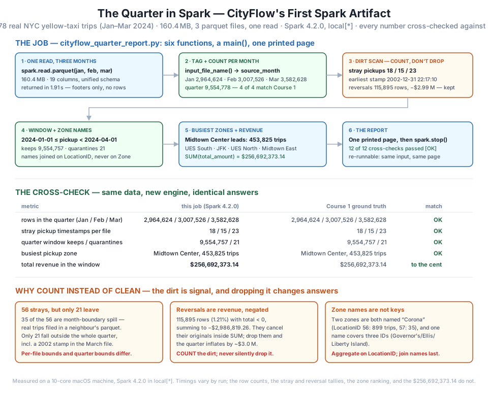
read.parquet pulls all 9,554,778 trips (160.4 MB, 3 files) into a single 19-column DataFrame — returning in 1.91 s because it read footers, not rows — and input_file_name() lets every row answer for its source file, so the per-month counts check against Course 1 exactly. The dirt census is reproduced in Spark rather than assumed: 18/15/23 stray stamps per file (56 total, of which 35 are month-boundary spill and only 21 leave the quarter — the earliest, 2002-12-31 22:17:10, hiding in the March file), plus 115,895 fare reversals worth −$2,986,819.26 that are counted and kept because they cancel inside SUM. Zones aggregate on LocationID — two zones are both named “Corona” and one name spans three IDs — and the ranking and revenue land on Course 1's numbers to the trip and to the cent: $256,692,373.14. Twelve cross-checks, twelve [OK]s, one re-runnable script.These extend the project. Keep cityflow_quarter_report.py and the four data files exactly as they are.
Exercise 1 — Find the two genuine duplicates. Course 1’s ground truth distinguishes reversals (repeated business keys with opposite amounts — over 30,000 per month, keep them) from genuine full-row duplicates: identical in all 19 columns, and there are exactly Jan 0 / Feb 2 / Mar 0 of them. Reproduce that census in Spark: for each source month, count the rows that are exact copies of another row, and print the February pair in full.
Hint
The cheap census is a subtraction: tagged.groupBy(“source_month”).count() versus the same on tagged.dropDuplicates() — but be careful which columns define “duplicate”: you must include all 19 data columns and the source_month tag (a Jan trip copied into the Feb file would be a cross-file coincidence, not a duplicate). To see the actual rows, groupBy all columns, count, and filter count > 1. Expect exactly one February group with count 2 — and notice the census would be off by thousands if you had keyed on the trip’s business columns only, which is precisely the reversal trap wearing a different hat.
Exercise 2 — Add a per-month revenue section to the report. Extend build_report() with three lines — January, February, March revenue inside the quarter window — plus a check that the three sum to the quarter’s $256,692,373.14. One design decision matters: should a row’s month come from its source file or from its pickup timestamp? The 35 spill rows from Step 6 make the two definitions differ.
Hint
Group the windowed frame by calendar month — F.date_trunc(“month”, F.col(“tpep_pickup_datetime”)) — not by source_month: a trip picked up at 00:00 on Feb 1 but filed in the January parquet belongs to February’s revenue, and grouping by file would misplace all 35 spill rows. Sum the three floats in Python and compare after formatting to two decimals, exactly as the script’s revenue check does; comparing raw float64 values for equality will fail on the last bits even when the cents agree.
Exercise 3 — Profile the column this project deliberately ignored. trip_distance is the quarter’s dirtiest column — Course 1 clocked its maximum at over 312,722 miles. Give the report a distance section: min, median, 99th percentile, and max per month, plus a count of trips claiming more than 100 miles. Decide — and write down — whether the report should flag them, cap them, or keep them as-is, and defend the choice in one sentence.
Hint
F.percentile_approx(“trip_distance”, [0.5, 0.99]) gets the quantiles in one pass; F.min/F.max ride along in the same agg. Expect an enormous gap between the 99th percentile (around 20 miles) and the max — that gap, not the max alone, is the evidence of dirt. The defensible policy for this report follows the reversal precedent: count and display, don’t mutate — distance doesn’t feed any number on the page, so silently capping it would add a data-altering step with no consumer. The moment a distance-weighted metric joins the report, the decision must be revisited — which is why it belongs written down.
You shipped CityFlow’s first Spark artifact and made it prove itself against an answer key. One multi-path read.parquet pulled all three months — 9,554,778 rows, 160.4 MB — into a single 19-column DataFrame, returning in 1.91 s because it read footers rather than rows, while count() did the real 9.5-million-row scan. input_file_name() attributed every row to its source file, and the per-month counts — 2,964,624 / 3,007,526 / 3,582,628 — matched Course 1 exactly. The sanity scan reproduced the known dirt in the new engine: 18/15/23 stray timestamps per file, with the quarter’s earliest stamp (2002-12-31 22:17:10) hiding in the March file, something Course 1’s January-focused dive never revealed; the reconciliation showed 56 per-file strays but only 21 quarter-level quarantines, because 35 are month-boundary spill — real fares filed in a neighbour’s parquet. The reversal census found 115,895 negative-total rows (1.21%) worth −$2,986,819.26, counted and kept because they cancel inside SUM — dropping them would inflate the quarter by ~$3.0M. The zone ranking, aggregated on LocationID (two zones are both “Corona”, 899 and 35 trips; one island name covers three IDs), matched Course 1’s top five to the trip — Midtown Center 453,825 at the head — and skipping the window filter shifted four of the five counts by exactly one trip, the least debuggable kind of wrong. The revenue check landed on $256,692,373.14 to the cent, with the raw float64 sum (256692373.14026505) showing exactly how much noise nine million parallel additions cost. All of it now lives in cityflow_quarter_report.py — functions, a main(), a printed page with 12 of 12 live cross-checks, and spark.stop() at the end — generated in 4.7 s on a warm session.
spark.read.parquet(p1, p2, p3) unifies many files into one DataFrame with one schema; the call returns in seconds having read only footers, and the first action does the real scan.input_file_name() — per-row lineage for free: after files merge, every row can still answer “which file did I come from?”, which turns a total-only check (9,554,778) into a per-month reconciliation (4 of 4 exact).SUM but inflate revenue by ~$3.0M if deleted; 35 of 56 “stray” timestamps are valid quarter rows. Every cleaning decision changes an answer, so a first-look job reports and preserves.Zone fuses them irrecoverably, while grouping by LocationID and joining for display matched Course 1 trip for trip.Every data team eventually migrates something — pandas to Spark, one warehouse to another, a vendor’s numbers to in-house numbers — and the migrations that go wrong don’t usually fail loudly. They produce plausible numbers: a quarter total that looks right, a ranking with familiar names in a familiar order, revenue in the right hundreds of millions. The only defense is the one this project practiced end to end: carry the old system’s verified numbers into the new system as executable checks, at the finest grain you can afford — not “about 9.5 million rows” but 2,964,624 in January, not “roughly $257M” but $256,692,373.14, printed next to an [OK] that a human didn’t produce. The dirt matters just as much as the totals, because dirt is where silent divergence hides: an engine that “helpfully” drops nulls, a filter someone added to make negatives go away, a join on a name that merges two Coronas — each one moves an answer while every schema check still passes. CityFlow’s first Spark job earns trust the only way trust is earned in this field: by being checkably, reproducibly right about data it didn’t choose and defects it didn’t cause. That’s the standard every artifact in the rest of this course is held to.
That completes Module 1: Why Distributed? — the ceiling of one machine measured honestly, Spark’s driver-and-executor architecture, your first SparkSession, the unflattering truth about small data, and now a real artifact that cross-checks a new engine against a verified quarter, twelve for twelve.
But this project left a mystery sitting in plain sight, back in Step 2. read.parquet on 160 MB returned in under two seconds without reading a single trip — and then count(), groupBy, and every check after it each went back to the files and did real work, sometimes re-reading data a previous step had already touched. Why does Spark hand you a DataFrame it hasn’t materialized? Why is that not a bug but the entire design? Module 2 — SparkSession, RDDs & Lazy Evaluation — opens the hood: what a DataFrame actually is underneath (an RDD and a plan), why Spark refuses to compute anything until an action forces it, how it fuses your chain of transformations into optimized stages, and when you should — and shouldn’t — cache the results. Once you can read Spark’s plans, the timings in this module stop being curiosities and become things you can predict.
Keep DATATWEETS free. Help fund practical data, AI, and engineering lessons for learners worldwide.
