Title here
Summary here
Go back to Module 1 for a moment. A single 50 MB file expanded to roughly 400 MB the instant pandas touched it, and that was the whole problem in miniature: the data was small, the machine was large, and the obvious approach still fell over. Every module since has been one answer to that problem. Module 2 made the numbers themselves smaller. Module 3 made pandas lean. Module 4 stopped loading the file at all and streamed it into a warehouse. Module 5 put every core to work. Module 6 replaced scans with the right container. Module 7 restored the order that hashing throws away, so a range could be answered without reading everything. Each module left one reusable piece, and each piece was measured rather than asserted.
This project stacks them into a single pipeline. CityFlow’s dashboard team needs a per-zone, per-hour trip and revenue report over a full quarter — three months of real yellow-taxi data, 9,554,778 trips, 160 MB on disk that becomes 1,347 MB the moment you materialize it in pandas. A naive read_parquet and groupby produces the right answer and needs nearly a gigabyte of RAM to do it. Your pipeline will produce the same answer — to the cent — under a declared 400 MB budget, and its peak memory will barely move as you add months while the naive path climbs past 900 MB.
The harder half is the data, and this is where the project stops being a tidy exercise. This dataset is genuinely defective in ways that punish a careless pipeline: tens of thousands of repeated keys that are accounting reversals rather than duplicates, so deduplicating them overstates revenue; timestamps stamped 2002 and 2009 sitting in a 2024 file, few enough to shrug at and destructive enough to ruin an index; zone names that are not unique, so a join on the wrong column silently loses trips. A pipeline that is fast and wrong is worth nothing, and the last thing this course will teach you is how to know the difference. Let’s build one that is neither.
By the end of this project, you will be able to:
You’ll need pandas, numpy, pyarrow, and the standard library (sqlite3, multiprocessing, resource). Everything runs on real data, for real.
Before writing a pipeline, write down what “done” means. CityFlow’s report has to satisfy five things, and we will check every one of them against real output rather than trusting the code:
(zone, hour) table of trip counts and revenue over Q1 2024, and it must equal what a dumb full-load baseline produces — exactly, not approximately.Here is the setup — the file list, the three columns we actually need, the reporting window, the budget, and the zone dimension. Note the very first data-quality decision, made before a single trip is read: the zone dimension is keyed on LocationID, never on the zone name.
# gate: skip
# CityFlow's three months of yellow-taxi trips, fetched once from the public NYC TLC site.
# (The gate reads the already-staged local copies; this block documents where they come from.)
import urllib.request
base = "https://d37ci6vzurychx.cloudfront.net/trip-data/"
for name in ["yellow_tripdata_2024-01.parquet",
             "yellow_tripdata_2024-02.parquet",
             "yellow_tripdata_2024-03.parquet"]:
    urllib.request.urlretrieve(base + name, name)
import warnings; warnings.filterwarnings("ignore")
import time, os, sys, sqlite3, resource
import datetime as dt
import multiprocessing as mp
import numpy as np
import pandas as pd
import pyarrow as pa
import pyarrow.parquet as pq
FILES = ["yellow_tripdata_2024-01.parquet",
"yellow_tripdata_2024-02.parquet",
"yellow_tripdata_2024-03.parquet"]
KEEP = ["tpep_pickup_datetime", "PULocationID", "total_amount"]
WIN_LO = dt.datetime(2024, 1, 1)
WIN_HI = dt.datetime(2024, 4, 1)
BUDGET_MB = 400
DB = "m8_warehouse.db"
def load_zones(path="taxi_zone_lookup.csv"):
"""Zone dimension: LocationID -> (Zone, Borough). Keyed on the ID, never the name."""
z = pd.read_csv(path)
return z.set_index("LocationID")[["Zone", "Borough"]]
if __name__ == "__main__":
ZONES = load_zones()
print(f"zone dimension rows : {len(ZONES)}")
dupe_names = ZONES[ZONES.duplicated('Zone', keep=False)].dropna(subset=['Zone'])
print(f"zone NAMES that are not unique: {dupe_names['Zone'].nunique()} names, {len(dupe_names)} ids")
print(dupe_names.reset_index().to_string(index=False))zone dimension rows : 265
zone NAMES that are not unique: 2 names, 5 ids
LocationID Zone Borough
56 Corona Queens
57 Corona Queens
103 Governor's Island/Ellis Island/Liberty Island Manhattan
104 Governor's Island/Ellis Island/Liberty Island Manhattan
105 Governor's Island/Ellis Island/Liberty Island ManhattanThere it is, before we have read a single trip: five zone ids share two names. Queens has two entirely distinct zones both called “Corona” (LocationID 56 and 57), and Manhattan has three sharing one island name. If the report grouped trips by zone name, those would silently collapse into each other and the counts would be wrong with no error to warn you — the exact bug Module 7’s Lesson 1 hit when a recursive tree keyed its leaves on the name and lost 270 trips. Keying on LocationID and joining the name back last, for display only, is the fix. The whole pipeline carries this discipline.
Module 1’s rule was: measure before you optimize. So the first thing the pipeline does is quantify what the naive approach would cost, and turn that into the budget everything else must respect. We read one month to learn the real bytes-per-row in pandas, then extrapolate to all three.
if __name__ == "__main__":
    disk = sum(os.path.getsize(f) for f in FILES)
    rows_per_file = {f: pq.ParquetFile(f).metadata.num_rows for f in FILES}
    total_rows = sum(rows_per_file.values())
    sample = pq.read_table(FILES[0]).to_pandas()
    bytes_per_row = sample.memory_usage(deep=True).sum() / len(sample)
    materialized = bytes_per_row * total_rows / 1e6
    del sample
    print(f"{'file':<34}{'rows':>12}{'row groups':>12}")
    for f in FILES:
        md = pq.ParquetFile(f).metadata
        print(f"{f:<34}{md.num_rows:>12,}{md.num_row_groups:>12}")
    print(f"{'TOTAL':<34}{total_rows:>12,}")
    print(f"\non disk (3 files)              : {disk/1e6:.1f} MB")
    print(f"if fully materialized in pandas: {materialized:,.0f} MB  "
          f"({materialized/(disk/1e6):.1f}x the file size)")
    print(f"declared memory BUDGET         : {BUDGET_MB} MB  -- the pipeline must stay under this")
file rows row groups
yellow_tripdata_2024-01.parquet 2,964,624 3
yellow_tripdata_2024-02.parquet 3,007,526 3
yellow_tripdata_2024-03.parquet 3,582,628 4
TOTAL 9,554,778
on disk (3 files) : 160.4 MB
if fully materialized in pandas: 1,347 MB (8.4x the file size)
declared memory BUDGET : 400 MB -- the pipeline must stay under thisThe same 8.4x blow-up Module 1 measured on one file holds across three: 160 MB of Parquet becomes 1,347 MB in pandas, because Parquet stores columns compressed and typed tightly while pandas expands them into full-width objects and adds per-column overhead. Loading all three months at once to group them would need well over a gigabyte of working memory. We set the budget at 400 MB — comfortably above what a streaming pipeline needs, comfortably below what the naive load demands — and hold everything to it. (On this machine 1.3 GB happens to fit in RAM, so “out-of-core” here is enforced by the budget, not by a hard failure. That is deliberate: the property we are about to prove — flat memory as data grows — is exactly what lets the same code survive data that genuinely does not fit.)
This is the heart of the pipeline, and it folds three modules into one function. Module 4 said: never hold the whole file — read it a row group at a time. Modules 2 and 3 said: keep only the columns you need, in the smallest honest dtype. Module 5 (next step) will say: let each worker read its own partition rather than being handed a pickled DataFrame. So the unit of work is a (path, row_group) tuple, and the worker reads that one row group, keeps three of the file’s nineteen columns, filters junk, and returns a tiny aggregate — not rows.
def aggregate_partition(task):
    """M5 worker: takes (path, row_group) and reads ITS OWN partition -- never a pickled frame.
    Streams the row group (M4), keeps 3 columns (M2/M3), filters junk, returns a tiny aggregate."""
    path, rg = task
    tbl = pq.ParquetFile(path).read_row_group(rg, columns=KEEP)
    ts = tbl.column(0).to_numpy(zero_copy_only=False)          # datetime64[us]
    keep = (ts >= np.datetime64(WIN_LO)) & (ts < np.datetime64(WIN_HI))
    quarantined = int((~keep).sum())
    hour = ts[keep].astype("datetime64[h]").astype("int64")    # hours since epoch
    zone = tbl.column(1).to_numpy()[keep]                      # int32 PULocationID
    amt = tbl.column(2).to_numpy(zero_copy_only=False)[keep]   # float64 total_amount
    part = (pd.DataFrame({"zone": zone, "hour": hour, "amt": amt})
            .groupby(["zone", "hour"], sort=False)
            .agg(trips=("amt", "size"), revenue=("amt", "sum"))
            .reset_index())
    return part, quarantined


def tasks_for(files):
    return [(f, i) for f in files for i in range(pq.ParquetFile(f).metadata.num_row_groups)]


def reduce_parts(parts):
    agg = pd.concat([p for p, _ in parts], ignore_index=True)
    final = (agg.groupby(["zone", "hour"], sort=False)
             .agg(trips=("trips", "sum"), revenue=("revenue", "sum"))
             .reset_index())
    final["zone"] = final["zone"].astype("int64")
    return final, sum(q for _, q in parts)


if __name__ == "__main__":
    one = aggregate_partition((FILES[0], 0))[0]
    preview = one.head(3).copy()
    preview["hour"] = preview["hour"].values.astype("datetime64[h]")   # decode for display
    print("one row group (1,048,576 rows) reduced to aggregate rows:", f"{len(one):,}")
    print(preview.to_string(index=False))
    print("what travels back to the driver:", f"{one.memory_usage(deep=True).sum()/1e3:.0f} KB",
          "-- an aggregate, never a million-row frame")
one row group (1,048,576 rows) reduced to aggregate rows: 28,394
zone hour trips revenue
186 2024-01-01 97 3573.82
140 2024-01-01 71 1481.76
236 2024-01-01 141 2760.91
what travels back to the driver: 795 KB -- an aggregate, never a million-row frameA row group of 1,048,576 trips collapses to 28,394 aggregate rows — one per (zone, hour) bucket that appears in it — and only 795 KB crosses back to the caller. That collapse is the entire trick that makes parallelism cheap in the next step: because each worker returns a small aggregate instead of its million rows, there is nothing large to pickle and ship between processes, which is precisely the serialization trap Module 5 warned about. The map (aggregate each partition) and reduce (sum the partial aggregates) is the map-reduce shape from Module 5, and reduce_parts is the combine.
One subtlety hides in to_numpy() on the timestamp column: this data is datetime64[us] — microseconds, not nanoseconds. Comparing it against a Python datetime via np.datetime64 is safe, but if you had reached for pd.Timestamp(...).value (which returns nanoseconds) the comparison would have silently been off by a factor of a thousand and matched zero rows. Always check the unit before you trust an integer timestamp.
Now the substance. This dataset is dirty in specific, revenue-changing ways, and a pipeline that ignores them is confidently wrong. We scan each month for four things at once: how many business keys repeat, how many timestamps fall outside the month’s own window, how many repeats are reversals (the fare or total cancels to zero), and how many are genuine full-row duplicates. Crucially, we check every month rather than assuming January’s profile generalizes.
KEY5 = ["VendorID", "tpep_pickup_datetime", "tpep_dropoff_datetime", "PULocationID", "DOLocationID"]


def quality_scan(path, lo, hi):
    df = pq.read_table(path, columns=KEY5 + ["fare_amount", "total_amount"]).to_pandas()
    ts = df["tpep_pickup_datetime"]
    out_of_window = int(((ts < lo) | (ts >= hi)).sum())
    g = df[df.duplicated(KEY5, keep=False)].groupby(KEY5, sort=False)
    agg = g.agg(fsum=("fare_amount", "sum"), fabs=("fare_amount", lambda s: s.abs().sum()),
                tsum=("total_amount", "sum"), tabs=("total_amount", lambda s: s.abs().sum()))
    fare_rev = ((agg.fsum.abs() < 0.01) & (agg.fabs > 0.01)).sum()
    tot_rev = ((agg.tsum.abs() < 0.01) & (agg.tabs > 0.01)).sum()
    only_total = int((((agg.tsum.abs() < 0.01) & (agg.tabs > 0.01)) &
                      ~((agg.fsum.abs() < 0.01) & (agg.fabs > 0.01))).sum())
    identical = int(df.duplicated(keep=False).sum())
    return dict(rows=len(df), repeated_keys=len(agg), out_of_window=out_of_window,
                fare_rev=int(fare_rev), total_rev=int(tot_rev), only_total=only_total,
                identical=identical)


if __name__ == "__main__":
    windows = {"2024-01": (dt.datetime(2024,1,1), dt.datetime(2024,2,1)),
               "2024-02": (dt.datetime(2024,2,1), dt.datetime(2024,3,1)),
               "2024-03": (dt.datetime(2024,3,1), dt.datetime(2024,4,1))}
    print(f"{'month':<9}{'rows':>11}{'rep.keys':>10}{'out-win':>9}"
          f"{'fare-rev':>10}{'tot-rev':>9}{'only-tot':>10}{'identical':>10}")
    for m, f in zip(windows, FILES):
        lo, hi = windows[m]
        r = quality_scan(f, lo, hi)
        print(f"{m:<9}{r['rows']:>11,}{r['repeated_keys']:>10,}{r['out_of_window']:>9}"
              f"{r['fare_rev']:>10,}{r['total_rev']:>9,}{r['only_total']:>10}{r['identical']:>10}")
month rows rep.keys out-win fare-rev tot-rev only-tot identical
2024-01 2,964,624 31,109 18 30,980 30,676 120 0
2024-02 3,007,526 31,632 15 31,546 31,190 79 2
2024-03 3,582,628 38,904 23 38,766 38,395 133 0Read this table carefully, because it is the whole argument for why data quality is judgment and not a checkbox. Each month has tens of thousands of repeated business keys — 31,109 in January — and the instinct is to call those duplicates and drop them. They are not. In January, 30,980 of them have a fare_amount that sums to zero (a positive charge and an equal negative one) and another 120 have a zero fare whose money moves in total_amount instead; together, essentially all 31,109 are accounting reversals — a charge voided and rebilled, exactly as a ledger records a correction. The column that actually answers “is this a duplicate trip?” is identical: full rows that appear twice. For January it is 0. There are no genuine duplicates at all.
And here is why checking every month mattered: February’s identical count is 2, not 0. January’s clean result did not generalize. Two full rows really are replayed in February, and a pipeline that hard-coded “this dataset has no duplicates” from January would carry them silently into every total. March is back to zero. The lesson is the one this whole course keeps returning to: verify on the data in front of you, not on what a previous slice happened to show. (The out-win column carries a parallel warning — 18, 15, and 23 stray timestamps per month, some stamped 2002 and 2009, which is why the aggregator filters to an explicit window rather than trusting the file’s name.)
The reversals are not a curiosity; mishandling them moves the revenue number by six figures. Watch what happens if you “clean” the data with drop_duplicates on the business key — and notice that the direction of the error depends on an arbitrary keep= flag.
if __name__ == "__main__":
    print(f"{'month':<9}{'keep all':>16}{'drop KEY first':>18}{'drop KEY last':>18}{'drop full-row':>16}")
    for m, f in zip(windows, FILES):
        lo, hi = windows[m]
        df = pq.read_table(f, columns=KEY5 + ["total_amount"]).to_pandas()
        df = df[(df.tpep_pickup_datetime >= lo) & (df.tpep_pickup_datetime < hi)]
        allrev = df.total_amount.sum()
        first = df.drop_duplicates(KEY5, keep="first").total_amount.sum()
        last = df.drop_duplicates(KEY5, keep="last").total_amount.sum()
        full = df.drop_duplicates(keep="first").total_amount.sum()
        print(f"{m:<9}{allrev:>16,.0f}{first-allrev:>+18,.0f}{last-allrev:>+18,.0f}{full-allrev:>+16,.2f}")
month keep all drop KEY first drop KEY last drop full-row
2024-01 79,455,942 -787,612 +784,614 +0.00
2024-02 80,073,234 -811,602 +808,432 -23.16
2024-03 97,162,290 -1,033,941 +1,030,098 +0.00Keeping every row gives January’s true revenue: $79,455,942. Deduplicating on the key with keep="first" swings it down $787,612; keep="last" swings it up $784,614 — the same data, a swing of over $1.5 million, decided by nothing but which row of each reversal pair pandas happens to keep. The reason is simple once you see it: a reversal is a +X and a −X that sum to zero, so keeping all rows lets them cancel correctly, but keeping only one of the pair leaves an uncancelled +X or −X in the total. The right operation is to keep everything and let SUM cancel the reversals — which is exactly what the streaming aggregator already does. The last column confirms it from the other side: dropping only genuinely identical full rows changes January by $0.00 (there are none) and February by exactly −$23.16 (the two real duplicates, correctly removed). Data quality here is not “remove duplicates”; it is knowing that these are not duplicates.
The most expensive line of code is the one that looks harmless
df.drop_duplicates(KEY5) is a line a reviewer would wave through. On this data it silently rewrites revenue by more than a million dollars a month, in a direction set by a default argument. The pipeline never calls it. Preserving the reversals and summing is both simpler and correct — the fast path and the right path are the same path here, but only because someone looked at the rows first.
Ten row groups across three months, ten independent units of work, ten cores available. Module 5’s tools apply directly. But Module 5 also taught that you must measure a parallelism strategy rather than assume it, and this pipeline is a case where the assumption everyone brings is wrong. We race the same aggregation three ways: serial, six threads, six processes.
from concurrent.futures import ThreadPoolExecutor

if __name__ == "__main__":
    tasks = tasks_for(FILES)
    print("partitions (row groups across 3 months):", len(tasks))

    _ = [aggregate_partition(t) for t in tasks]                 # warm the page cache
    t0 = time.perf_counter(); serial = [aggregate_partition(t) for t in tasks]
    t_serial = time.perf_counter() - t0

    t0 = time.perf_counter()
    with ThreadPoolExecutor(max_workers=6) as ex:
        threaded = list(ex.map(aggregate_partition, tasks))
    t_thread = time.perf_counter() - t0

    t0 = time.perf_counter()
    with mp.Pool(processes=6) as pool:
        pooled = pool.map(aggregate_partition, tasks)
    t_proc = time.perf_counter() - t0

    print(f"serial       : {t_serial:5.2f} s   1.00x")
    print(f"threads(6)   : {t_thread:5.2f} s   {t_serial/t_thread:4.2f}x")
    print(f"processes(6) : {t_proc:5.2f} s   {t_serial/t_proc:4.2f}x")
    report, quarantined = reduce_parts(pooled)
    print(f"\naggregate buckets (zone x hour): {len(report):,}")
    print(f"trips kept: {int(report.trips.sum()):,}   quarantined (outside the quarter): {quarantined}")
partitions (row groups across 3 months): 10
serial : 0.29 s 1.00x
threads(6) : 0.17 s 1.75x
processes(6) : 0.80 s 0.37x
aggregate buckets (zone x hour): 240,917
trips kept: 9,554,757 quarantined (outside the quarter): 21This is the opposite of Module 5’s headline result, and it is worth sitting with rather than smoothing over. In Module 5, a heavy per-row Python loop ran 3.96x faster across processes and flat across threads, because the loop held the GIL and only separate processes could run it in parallel. Here, threads win (1.75x) and processes actually lose (0.37x — more than twice as slow as serial). Nothing contradicts Module 5; this is the other half of its rule. The work in aggregate_partition is almost entirely pyarrow’s Parquet decode and pandas’ groupby, both of which run in C and release the GIL while they work — so threads genuinely overlap, exactly as Module 5 said I/O-bound and C-heavy work would. Processes, meanwhile, pay to spawn six fresh interpreters and re-import the module, and for a job this short (0.29 s serial) that startup cost dwarfs the gain. The rule Module 5 actually taught was never “processes are faster” — it was “measure, because the answer depends on whether your hot loop holds the GIL.” This pipeline holds it in C, so threads are right. We keep the process pool in the final module for the case where per-partition work is heavier, but the honest reading of this measurement is that threads were the better tool.
The aggregation itself is done: 240,917 distinct (zone, hour) buckets, 9,554,757 trips kept, and 21 quarantined for falling outside the quarter — the dirty 2002/2009 timestamps, caught exactly where they should be.
The pipeline is fast, streaming, parallel, and full of careful data-quality decisions. None of that is worth anything if the answer is wrong. So we build the report a second time, the dumbest possible way — load all three months into one giant DataFrame and group it — and demand that the two agree.
def naive_report(files):
    big = pd.concat([pq.read_table(f, columns=KEEP).to_pandas() for f in files], ignore_index=True)
    ts = big["tpep_pickup_datetime"]
    big = big[(ts >= WIN_LO) & (ts < WIN_HI)]
    big["hour"] = big["tpep_pickup_datetime"].values.astype("datetime64[h]").astype("int64")
    out = (big.groupby(["PULocationID", "hour"], sort=False)
           .agg(trips=("total_amount", "size"), revenue=("total_amount", "sum"))
           .reset_index().rename(columns={"PULocationID": "zone"}))
    out["zone"] = out["zone"].astype("int64")
    return out


if __name__ == "__main__":
    naive = naive_report(FILES)
    a = report.sort_values(["zone", "hour"]).reset_index(drop=True)
    b = naive.sort_values(["zone", "hour"]).reset_index(drop=True)
    identical = (len(a) == len(b) and a["zone"].equals(b["zone"])
                 and a["hour"].equals(b["hour"]) and a["trips"].equals(b["trips"])
                 and np.allclose(a["revenue"], b["revenue"]))
    print("pipeline aggregate == naive baseline:", identical)
    print(f"both report {len(a):,} buckets, {int(a.trips.sum()):,} trips, "
          f"${a.revenue.sum():,.2f} revenue")
pipeline aggregate == naive baseline: True
both report 240,917 buckets, 9,554,757 trips, $256,692,373.14 revenueIdentical. The streaming, chunked, parallel pipeline and the brute-force full load agree on every one of the 240,917 buckets, all 9,554,757 trips, and the revenue to the cent: $256,692,373.14. This is the check that licenses everything else — the memory savings you are about to see are only worth having because the answer underneath them is provably the same one the simple approach would give. A pipeline that is 10x leaner and 0.001% wrong is not an optimization; it is a bug with good performance numbers.
Module 4 introduced SQLite as a local warehouse: a real, indexed, SQL-queryable store that lives in one file and holds far more than memory. The 240,917-row report is small, but the pattern is what matters — and the property that matters most for a pipeline is idempotency. Pipelines get retried after failures, so loading the same batch twice must not double-count. We enforce that with a primary key on (zone, hour) and INSERT OR REPLACE.
def build_warehouse(report, db=DB, timed=False):
    if os.path.exists(db):
        os.remove(db)
    con = sqlite3.connect(db)
    con.execute("""CREATE TABLE zone_hour (zone INTEGER, hour INTEGER,
                   trips INTEGER, revenue REAL, PRIMARY KEY (zone, hour)) WITHOUT ROWID""")
    t0 = time.perf_counter(); load_warehouse(con, report); t_load = time.perf_counter() - t0
    t0 = time.perf_counter()
    con.execute("CREATE INDEX ix_zone_hour_hour ON zone_hour(hour)")
    con.commit(); t_index = time.perf_counter() - t0
    if timed:
        print(f"  load {len(report):,} rows into SQLite : {t_load*1000:6.0f} ms")
        print(f"  build the secondary B-tree index : {t_index*1000:6.0f} ms")
    return con


def load_warehouse(con, report):
    """Idempotent: keyed on (zone, hour) with INSERT OR REPLACE, re-running never double-counts."""
    rows = list(report[["zone", "hour", "trips", "revenue"]]
                .astype({"zone": "int64", "hour": "int64", "trips": "int64"})
                .itertuples(index=False, name=None))
    con.executemany("INSERT OR REPLACE INTO zone_hour VALUES (?,?,?,?)", rows)
    con.commit()


if __name__ == "__main__":
    con = build_warehouse(report, timed=True)
    before = con.execute("SELECT COUNT(*), SUM(trips), ROUND(SUM(revenue),2) FROM zone_hour").fetchone()
    load_warehouse(con, report)          # run the SAME load again
    after = con.execute("SELECT COUNT(*), SUM(trips), ROUND(SUM(revenue),2) FROM zone_hour").fetchone()
    print("after first load :", before)
    print("after re-running :", after)
    print("idempotent (no double-count):", before == after)
    print("warehouse on disk:", f"{os.path.getsize(DB)/1e6:.2f} MB")
load 240,917 rows into SQLite : 290 ms
build the secondary B-tree index : 53 ms
after first load : (240917, 9554757, 256692373.14)
after re-running : (240917, 9554757, 256692373.14)
idempotent (no double-count): True
warehouse on disk: 8.16 MBLoading the same report a second time leaves every total untouched: 240,917 rows, 9,554,757 trips, $256,692,373.14 both before and after. Because each (zone, hour) is a primary key, the second load replaces rows rather than appending them — so a retried or double-triggered pipeline run is safe, which is the difference between a warehouse you can operate and one you have to babysit. The whole quarter of aggregates sits in an 8.16 MB file.
Modules 6 and 7 were about answering a question without scanning everything: a hash for exact match, ordered keys for ranges. SQLite gives us both for free through indexes, which are B-trees — the ordered, shallow, cache-friendly trees Module 7 pointed at when it noted that real databases ship B-trees rather than hand-rolled BSTs. The primary key on (zone, hour) answers per-zone questions; the secondary index on hour answers per-hour ranges. We can watch the query planner choose them, and measure what they buy against an unindexed copy.
if __name__ == "__main__":
    plan_zone = con.execute("EXPLAIN QUERY PLAN "
                            "SELECT SUM(trips) FROM zone_hour WHERE zone=132").fetchone()[-1]
    plan_hour = con.execute("EXPLAIN QUERY PLAN SELECT zone, SUM(trips) FROM zone_hour "
                            "WHERE hour BETWEEN ? AND ? GROUP BY zone", (0, 0)).fetchone()[-1]
    print("per-zone plan:", plan_zone)
    print("per-hour plan:", plan_hour)

    # a bare copy WITHOUT the primary-key index, to show what the index buys
    con.execute("CREATE TABLE zh_noidx AS SELECT * FROM zone_hour")
    con.commit()

    def timeit(sql, args=(), n=200):
        con.execute(sql, args)
        t0 = time.perf_counter()
        for _ in range(n):
            con.execute(sql, args).fetchall()
        return (time.perf_counter() - t0) / n * 1000

    idx = timeit("SELECT SUM(trips), SUM(revenue) FROM zone_hour WHERE zone=?", (132,))
    scan = timeit("SELECT SUM(trips), SUM(revenue) FROM zh_noidx WHERE zone=?", (132,))
    print(f"\nper-zone read via PK B-tree : {idx*1000:7.1f} us")
    print(f"per-zone read, full scan    : {scan*1000:7.1f} us   ({scan/idx:.1f}x slower)")
    con.execute("DROP TABLE zh_noidx"); con.commit()
per-zone plan: SEARCH zone_hour USING PRIMARY KEY (zone=?)
per-hour plan: SEARCH zone_hour USING INDEX ix_zone_hour_hour (hour>? AND hour<?)
per-zone read via PK B-tree : 113.7 us
per-zone read, full scan : 5012.0 us (44.1x slower)SEARCH ... USING PRIMARY KEY and SEARCH ... USING INDEX — the planner confirms both reads walk a B-tree rather than scanning the table. The payoff is concrete: a per-zone read costs 113.7 µs against the index and 5,012 µs against an unindexed copy of the same rows — 44x. That is the same order of magnitude as Module 7’s hand-built index win (36,986x on a raw array was the range-slice extreme; 44x here is a full aggregate over one zone’s rows), and it comes essentially for free because SQLite maintains the tree as part of the primary key.
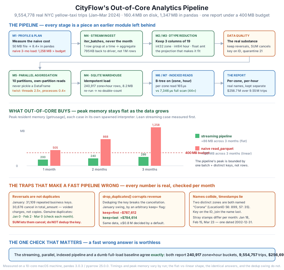
400 MB budget, while the naive read_parquet grows linearly and blows through it at every size — because the pipeline's footprint is bounded by one batch plus the distinct keys, not by the row count. The traps (band three) are all real and checked per month, including February's 2 genuine duplicates that January's 0 would have hidden. The check that matters (band four): pipeline and baseline agree exactly — 240,917 buckets, 9,554,757 trips, $256,692,373.14. Exact milliseconds and megabytes vary by run; the flat-versus-linear shape, the identical answers, and the dedup swing do not.Everything so far establishes that the pipeline is correct and fast. This step proves the property the whole course is named for: memory that stays flat as the data grows. We measure peak resident memory for the streaming pipeline and the naive load at one, two, and three months — each in its own freshly spawned interpreter, so no measurement inherits another’s high-water mark, and with the lean streaming cases run first. (ru_maxrss only ever increases within a process, so measurement order matters; running each case in a clean process is the honest way to compare.)
def peak_mb():
    kb = resource.getrusage(resource.RUSAGE_SELF).ru_maxrss
    return kb / (1024 * 1024) if sys.platform == "darwin" else kb / 1024


def stream_report(files, batch=131072):
    """The true out-of-core path: iter_batches (M4), a running dict aggregate
    whose size tracks distinct (zone, hour) keys (M6), never the row count."""
    acc = {}
    for f in files:
        for rec in pq.ParquetFile(f).iter_batches(batch_size=batch, columns=KEEP):
            ts = rec.column(0).to_numpy(zero_copy_only=False)
            keep = (ts >= np.datetime64(WIN_LO)) & (ts < np.datetime64(WIN_HI))
            hour = ts[keep].astype("datetime64[h]").astype("int64")
            zone = rec.column(1).to_numpy()[keep]
            amt = rec.column(2).to_numpy(zero_copy_only=False)[keep]
            part = (pd.DataFrame({"zone": zone, "hour": hour, "amt": amt})
                    .groupby(["zone", "hour"], sort=False)
                    .agg(t=("amt", "size"), r=("amt", "sum")))
            for (z, h), row in part.iterrows():
                k = (int(z), int(h))
                if k in acc:
                    acc[k][0] += int(row.t); acc[k][1] += float(row.r)
                else:
                    acc[k] = [int(row.t), float(row.r)]
    return pd.DataFrame([(z, h, v[0], v[1]) for (z, h), v in acc.items()],
                        columns=["zone", "hour", "trips", "revenue"])


def _floor(q): q.put(("imports only", peak_mb()))
def _stream(q, k): stream_report(FILES[:k]); q.put((f"streaming pipeline, {k} mo", peak_mb()))
def _naive(q, k): naive_report(FILES[:k]); q.put((f"naive read_parquet, {k} mo", peak_mb()))


if __name__ == "__main__":
    ctx = mp.get_context("spawn")
    mrows = []
    for fn, arg in [(_floor, None), (_stream, 1), (_stream, 2), (_stream, 3),
                    (_naive, 1), (_naive, 2), (_naive, 3)]:
        q = ctx.Queue()
        args = (q,) if arg is None else (q, arg)
        p = ctx.Process(target=fn, args=args); p.start(); mrows.append(q.get()); p.join()
    floor = mrows[0][1]
    print(f"{'variant':<28}{'peak RSS':>10}{'over floor':>12}{'vs 400MB budget':>17}")
    for name, mb in mrows:
        flag = "UNDER" if mb < BUDGET_MB else "OVER budget"
        print(f"{name:<28}{mb:>7.0f} MB{mb-floor:>9.0f} MB{flag:>17}")
variant peak RSS over floor vs 400MB budget
imports only 96 MB 0 MB UNDER
streaming pipeline, 1 mo 204 MB 108 MB UNDER
streaming pipeline, 2 mo 239 MB 143 MB UNDER
streaming pipeline, 3 mo 283 MB 187 MB UNDER
naive read_parquet, 1 mo 495 MB 399 MB OVER budget
naive read_parquet, 2 mo 861 MB 765 MB OVER budget
naive read_parquet, 3 mo 957 MB 861 MB OVER budgetThis is the payoff for the whole course. The naive load is already over the 400 MB budget at a single month (495 MB) and climbs to 957 MB at three — its footprint grows with the row count, because it holds every row in memory to group them. The streaming pipeline holds at 204, 239, 283 MB — under budget at every size, and growing only slowly as months are added. That slow growth is honest and worth explaining: the pipeline’s peak is bounded by one batch of rows plus the accumulating dictionary of distinct (zone, hour) keys (Module 6’s idea), and there are only ~240,000 such keys no matter how many trips flow through. It grows with the size of the answer, not the size of the input. That is precisely what lets this same code process a year, or ten years, on a laptop: add data and the memory barely moves. (Exact megabytes vary by run and machine; the flat-versus-linear shape does not.)
Finally, the artifact CityFlow keeps. Everything above collapses into one class: build runs the parallel aggregation and loads the warehouse; the query methods answer per-zone and per-hour questions off the B-tree, joining zone names back for display — by id, so the two Coronas stay distinct.
class ZoneHourWarehouse:
    """CityFlow's out-of-core analytics warehouse. build() streams+aggregates+loads;
    the query methods answer per-zone and per-hour questions off the B-tree index."""

    def __init__(self, db=DB, zones_csv="taxi_zone_lookup.csv"):
        self.con = sqlite3.connect(db)
        self.zones = load_zones(zones_csv)

    @classmethod
    def build(cls, files, db=DB, workers=6):
        tasks = [(f, i) for f in files for i in range(pq.ParquetFile(f).metadata.num_row_groups)]
        with mp.Pool(processes=workers) as pool:
            parts = pool.map(aggregate_partition, tasks)
        agg = pd.concat([p for p, _ in parts], ignore_index=True)
        report = (agg.groupby(["zone", "hour"], sort=False)
                  .agg(trips=("trips", "sum"), revenue=("revenue", "sum")).reset_index())
        con = build_warehouse(report, db)
        con.close()
        return cls(db)

    def _name(self, zone_id):
        try:
            r = self.zones.loc[zone_id]; return f"{r.Zone} ({r.Borough})"
        except KeyError:
            return f"zone {zone_id}"

    def zone_profile(self, zone_id):
        """M6: everything about one zone, straight off the (zone, hour) B-tree."""
        rows = self.con.execute(
            "SELECT hour%24 AS hod, SUM(trips), SUM(revenue) FROM zone_hour "
            "WHERE zone=? GROUP BY hod ORDER BY hod", (zone_id,)).fetchall()
        return pd.DataFrame(rows, columns=["hour_of_day", "trips", "revenue"])

    def top_zones(self, n=5):
        rows = self.con.execute(
            "SELECT zone, SUM(trips) t, SUM(revenue) r FROM zone_hour "
            "GROUP BY zone ORDER BY t DESC LIMIT ?", (n,)).fetchall()
        return [(z, self._name(z), t, r) for z, t, r in rows]

    def busiest_hours(self, n=5):
        rows = self.con.execute(
            "SELECT zone, hour, trips, revenue FROM zone_hour ORDER BY trips DESC LIMIT ?",
            (n,)).fetchall()
        return [(self._name(z), str(np.array(h, dtype="datetime64[h]")), t, r)
                for z, h, t, r in rows]


if __name__ == "__main__":
    con.close()
    wh = ZoneHourWarehouse.build(FILES)
    print("=== CityFlow Q1 2024 report (Jan-Mar, 3 months of yellow-taxi trips) ===\n")
    print("Busiest pickup zones over the quarter:")
    for zid, nm, t, r in wh.top_zones(5):
        print(f"  {nm:<40} {t:>10,} trips   ${r:>15,.2f}")
    print("\nBusiest single zone-hours in the quarter:")
    for nm, when, t, r in wh.busiest_hours(3):
        print(f"  {nm:<32} {when}   {t:>4} trips   ${r:>10,.2f}")
    prof = wh.zone_profile(132)
    peak = prof.loc[prof.trips.idxmax()]; low = prof.loc[prof.trips.idxmin()]
    print(f"\nJFK Airport hourly demand profile (132):")
    print(f"  busiest hour of day : {int(peak.hour_of_day):02d}:00  {int(peak.trips):,} trips")
    print(f"  quietest hour of day: {int(low.hour_of_day):02d}:00  {int(low.trips):,} trips")
    # two distinct 'Corona' zones -- keyed on ID, not name
    print("\nTwo distinct 'Corona' zones, kept separate because we keyed on LocationID:")
    for zid in (56, 57):
        t = wh.con.execute("SELECT SUM(trips) FROM zone_hour WHERE zone=?", (zid,)).fetchone()[0]
        print(f"  LocationID {zid}: {t:,} trips")
    wh.con.close()
=== CityFlow Q1 2024 report (Jan-Mar, 3 months of yellow-taxi trips) ===
Busiest pickup zones over the quarter:
Midtown Center (Manhattan) 453,825 trips $ 10,814,379.78
Upper East Side South (Manhattan) 439,138 trips $ 8,694,610.47
JFK Airport (Queens) 429,745 trips $ 33,137,512.96
Upper East Side North (Manhattan) 416,508 trips $ 8,477,163.42
Midtown East (Manhattan) 336,460 trips $ 7,829,595.20
Busiest single zone-hours in the quarter:
East Village (Manhattan) 2024-02-25T01 846 trips $ 17,891.31
East Village (Manhattan) 2024-02-25T00 803 trips $ 17,371.51
Midtown Center (Manhattan) 2024-02-29T17 779 trips $ 20,840.14
JFK Airport hourly demand profile (132):
busiest hour of day : 16:00 32,934 trips
quietest hour of day: 04:00 1,717 trips
Two distinct 'Corona' zones, kept separate because we keyed on LocationID:
LocationID 56: 899 trips
LocationID 57: 35 tripsThere is CityFlow’s report, built from three months of real trips under a 400 MB budget. Midtown Center is the quarter’s busiest pickup zone at 453,825 trips, with JFK Airport third by count but far ahead on revenue — $33.1 million, because airport runs are long. The busiest single hours are 1 a.m. in the East Village on February 25th (a Saturday-night-into-Sunday bar-close surge) and 5 p.m. in Midtown on February 29th — the leap day, a real date in a real month. JFK’s demand peaks at 4 p.m. and bottoms out at 4 a.m., exactly the airport-departure shape you would expect. And the two Corona zones report separately — 899 trips and 35 — because the pipeline keyed on LocationID from the very first step. Every number here traces back through the warehouse, the parallel aggregation, and the streaming ingest to the raw files, and every one of them survived the data’s defects because the pipeline was built to expect them.
if __name__ == "__main__":
    for f in os.listdir("."):
        if f.startswith("m8_"):
            os.remove(f)
    print("cleaned:", [f for f in os.listdir(".") if f.startswith("m8_")] or "no m8_ files left")
    print("staged datasets intact:",
          all(os.path.exists(f) for f in FILES + ["taxi_zone_lookup.csv", "yellow_tripdata_sample.csv"]))
cleaned: no m8_ files left
staged datasets intact: TrueExercise 1 — Add a fourth month and confirm the memory stays flat. Fetch yellow_tripdata_2024-04.parquet, add it to FILES, and re-run the memory measurement from Step 8 for one through four months. Confirm the streaming pipeline’s peak barely moves while the naive baseline’s climbs again, and report the new total trips and revenue. Then explain in a comment why the streaming peak grew a little even though “out-of-core” is supposed to be flat.
Hint
The streaming peak is bounded by one batch plus the dictionary of distinct (zone, hour) keys. April adds trips (which don’t accumulate — each batch is discarded) but also a few new keys for hours that didn’t appear before, and the dict holds those forever. The growth you see is the size of the answer growing, not the input; it is bounded by 265 zones times the number of distinct hours, not by the row count.
Exercise 2 — Make the reversals visible instead of silently correct. Extend aggregate_partition to also count, per (zone, hour), how many rows had a negative total_amount. Add a reversals column to the warehouse and find the zone-hours with the most reversals. Are they concentrated anywhere — a particular zone, a particular hour? Report what you find.
Hint
A negative total_amount is the void half of a reversal pair. Count (amt < 0).sum() alongside the trip count in the groupby. You are not removing them — they still cancel in the revenue sum — you are just surfacing them as a data-quality signal. If a zone-hour has an unusually high reversal rate, that is worth flagging to whoever owns the meter software.
Exercise 3 — Prove the idempotency claim the hard way. Load the warehouse, then load it again from a different month subset (say, only February’s aggregates) and confirm that February’s (zone, hour) rows are replaced, not doubled, while January’s and March’s are untouched. Then break it: change INSERT OR REPLACE to a plain INSERT and show the primary-key violation it raises. Explain why the WITHOUT ROWID primary key is what makes the safe version work.
Hint
INSERT OR REPLACE keyed on (zone, hour) means a second load of the same key overwrites in place — that is idempotency. A plain INSERT will raise sqlite3.IntegrityError: UNIQUE constraint failed on the first repeated key, which is SQLite refusing to double-count. Re-aggregating and replacing a single month’s keys is exactly how a real incremental pipeline reloads corrected data without touching the rest.
You built CityFlow’s out-of-core analytics pipeline end to end over 9,554,778 real trips across three months, and it satisfied every acceptance criterion. It profiled the naive cost (160 MB on disk, 1,347 MB in pandas — an 8.4x blow-up) and set a 400 MB budget; streamed the data a row group at a time, keeping three columns of nineteen and returning 795 KB aggregates instead of million-row frames; handled the data’s genuine defects by preserving 31,109 accounting reversals so their sums cancel (deduplicating them would have swung January’s revenue by over $1.5 million depending on an arbitrary flag), quarantining the 2002/2009 junk timestamps, catching February’s 2 real duplicates that January’s zero would have hidden, and keying on LocationID so the two distinct Corona zones stayed separate; aggregated in parallel, where measurement showed threads winning 1.75x and processes losing because the work releases the GIL in C — the honest other half of Module 5’s rule; loaded an idempotent SQLite warehouse that a retry cannot double-count; indexed it into a B-tree that answers per-zone reads 44x faster than a scan; and verified the whole thing against a full-load baseline, agreeing to the cent: 240,917 buckets, 9,554,757 trips, $256,692,373.14. Above all, it proved the property the course is named for — peak memory of 204-283 MB that stayed flat as months were added, while the naive path climbed from 495 MB to 957 MB.
drop_duplicates would have corrupted revenue by six figures in a direction set by a default. Checking every month caught February’s 2 genuine duplicates that January hid.Everything in this course was aimed at a single capability: engineering data that is bigger than the memory you have, on the hardware you have, correctly. This capstone is what that looks like assembled — not eight isolated techniques but one pipeline where each choice has a measured reason, the memory stays bounded as the data grows without bound, and the defects in real data are expected rather than discovered in production. The pattern generalizes far past taxi trips: profile before you optimize, stream instead of load, reduce before you compute, parallelize what genuinely parallelizes, warehouse the aggregates, index the reads, and never ship a number you have not checked against a simpler one. That discipline — and the habit of looking at the rows before trusting them — is the difference between a data engineer whose pipelines are fast and one whose pipelines are also right.
Look back at the whole course for a moment. In Module 1 a 50 MB file defeated a laptop; here, three months and nearly ten million trips flow through a pipeline that holds under 400 MB and answers to the cent. You did not get there with a bigger machine or a cloud bill — you got there by understanding where memory goes, choosing the right dtype and the right container, streaming instead of loading, using every core where it helps and knowing where it doesn’t, keeping data in order so ranges stay cheap, and refusing to trust a number you hadn’t verified. That is the core of data engineering, and you now have it, measured and in your hands.
This is also the end of the first course in CityFlow’s story, not the end of the story. Scaling Python for Data Engineering taught you to make one machine do far more than it looks capable of. The path from here goes outward: PySpark for Data Engineering takes the same map-reduce and partitioning ideas you used with multiprocessing.Pool and scales them across a cluster’s worth of executors, so the dataset can outgrow not just memory but the whole machine. After that, Docker & Kubernetes for Data Engineering makes these pipelines reproducible and deployable rather than laptop-bound, and Airflow turns them from scripts you run into schedules that run themselves. The taxi data, the CityFlow team, and the habits you built here carry straight into all three. You’ve finished the foundation — the part every distributed system is still built on top of.
Keep DATATWEETS free. Help fund practical data, AI, and engineering lessons for learners worldwide.
