Lesson 1 - The Chunking Idea

Welcome to The Chunking Idea#

So far at CityFlow you have made a DataFrame that is already in memory smaller: Module 3 downcast the taxi sample’s numeric columns and converted the repetitive ones to categoricals, cutting its footprint by more than half. Every one of those wins assumed the data fit in RAM in the first place. This module removes that assumption. A single month of NYC yellow-taxi trips is 2,964,624 rows, and when pandas loads all 19 of its columns the frame occupies about 399 MB. Load two months and you are past 800 MB; load a full year and an ordinary laptop simply cannot hold it. Downcasting helps, but it does not change the fundamental problem: you cannot narrow a frame you were never able to build.

The escape is to stop loading the whole file at all. Instead you stream it: read a small piece, do your work on that piece, keep only a tiny running result, and let the piece go before reading the next one. Peak memory then depends on the size of one piece, not the size of the file, so the same code that processes 200,000 rows processes 3 million or 30 million with an identical footprint. This lesson builds that mindset from the ground up, first on the sample CSV where you can watch every chunk, then on the real full-month parquet where it actually matters.

By the end of this lesson, you will be able to:

• Explain why loading a whole file into pandas ties peak memory to file size, and why that breaks at scale
• Use pd.read_csv(chunksize=...) to get an iterator of DataFrames and process every row without holding more than one chunk
• Measure that a single chunk’s memory footprint is a small, constant fraction of the whole-file footprint
• Stream a parquet file that does not comfortably fit in RAM with pyarrow’s iter_batches, counting all 2,964,624 rows with a tiny peak footprint
• State the streaming rule as a repeatable pattern: read a piece, do work, keep a small result, drop the piece

You will use pandas and pyarrow. Let’s start with the problem.

The Problem: Whole-File Loading Ties Memory to File Size#

CityFlow’s development sample is the 200,000-trip file you have used all course. It lives on the site here:

# gate: skip
# CityFlow's teaching sample: 200,000 real NYC yellow-taxi trips (~15 MB CSV).
import pandas as pd
taxi = pd.read_csv("https://datatweets.com/datasets/nyc-taxi/yellow_tripdata_sample.csv")

Download that file once and save it next to your script; every runnable block below reads the local copy by name. When you load it whole, pandas has to materialize all 200,000 rows and all 10 columns in memory at the same moment:

import warnings
warnings.filterwarnings("ignore")
import pandas as pd

taxi = pd.read_csv("yellow_tripdata_sample.csv")
whole = taxi.memory_usage(deep=True).sum()

print("rows:", f"{len(taxi):,}")
print("columns:", taxi.shape[1])
print(f"whole file in pandas: {whole:,} bytes  ({whole/1024/1024:.1f} MB)")

rows: 200,000
columns: 10
whole file in pandas: 23,600,132 bytes  (22.5 MB)

The 15 MB sample is 22.5 MB in pandas, and this is the small file — the one deliberately sized to fit anywhere. The full January parquet is 50 MB on disk and expands to about 399 MB in pandas because it carries all 19 real taxi columns for nearly 3 million rows. The relationship is the trap: peak memory scales with the file. Double the rows and you double the footprint, until one day the file is bigger than the RAM you have and read_csv fails with a MemoryError — after grinding for a while, at the worst possible time, in production. Downcasting shifts the ceiling a little higher; it does not remove the ceiling.

Reading a File in Chunks#

pd.read_csv has an argument that changes everything: chunksize. Give it a number of rows and it stops returning one DataFrame. Instead it returns an iterator that hands you the file one chunk at a time, each chunk a real DataFrame of at most chunksize rows. Nothing is read until you start iterating, and only one chunk is in memory at any moment:

import warnings
warnings.filterwarnings("ignore")
import pandas as pd

reader = pd.read_csv("yellow_tripdata_sample.csv", chunksize=50_000)
print("type of reader:", type(reader).__name__)

n_chunks = 0
total_rows = 0
for chunk in reader:
    n_chunks += 1
    total_rows += len(chunk)
    print(f"chunk {n_chunks}: {type(chunk).__name__}, {len(chunk):,} rows, columns={chunk.shape[1]}")

print(f"chunks seen: {n_chunks}")
print(f"total rows counted: {total_rows:,}")

type of reader: TextFileReader
chunk 1: DataFrame, 50,000 rows, columns=10
chunk 2: DataFrame, 50,000 rows, columns=10
chunk 3: DataFrame, 50,000 rows, columns=10
chunk 4: DataFrame, 50,000 rows, columns=10
chunks seen: 4
total rows counted: 200,000

Read that output slowly, because it contains the whole idea. The reader is not a DataFrame — it is a TextFileReader, an iterator. Looping over it produces four objects, and each one is a genuine DataFrame with the full 10 columns; you can call .groupby, .mean, or any other pandas method on it exactly as usual. There are four chunks because 200,000 rows divided by a chunksize of 50,000 is exactly 4. And the number that proves the technique is the last one: summing len(chunk) across the loop gives 200,000 — every single row was processed, none skipped, none seen twice — yet at no instant did the program hold more than 50,000 rows. You touched all the data while carrying a quarter of it.

If the row count did not divide evenly, the final chunk would simply be smaller (the remainder), and the row totals would still add up to the whole file. The loop body is where your real work goes: filter, aggregate, transform, write out. Whatever you do, you do it one chunk at a time.

The Memory Payoff: a Constant Footprint#

“A quarter of the rows” is the intuition; the number your team cares about is bytes. Measure the whole-file footprint against the peak footprint of any single chunk:

import warnings
warnings.filterwarnings("ignore")
import pandas as pd

whole = pd.read_csv("yellow_tripdata_sample.csv")
whole_mem = whole.memory_usage(deep=True).sum()

peak_chunk_mem = 0
for chunk in pd.read_csv("yellow_tripdata_sample.csv", chunksize=50_000):
    peak_chunk_mem = max(peak_chunk_mem, chunk.memory_usage(deep=True).sum())

print(f"whole file held at once: {whole_mem:,} bytes  ({whole_mem/1024/1024:.1f} MB)")
print(f"peak single chunk:       {peak_chunk_mem:,} bytes  ({peak_chunk_mem/1024/1024:.1f} MB)")
print(f"chunk footprint is {whole_mem/peak_chunk_mem:.1f}x smaller")

whole file held at once: 23,600,132 bytes  (22.5 MB)
peak single chunk:       5,900,132 bytes  (5.6 MB)
chunk footprint is 4.0x smaller

The peak chunk is 5.6 MB against the whole file’s 22.5 MB — almost exactly one quarter, because a chunk holds one quarter of the rows. But the fraction is not the important part. The important part is the word constant. That 5.6 MB is set by chunksize, not by the file. If the CSV had a million rows, you would still read it in 50,000-row chunks and the peak chunk would still be about 5.6 MB — you would just do more loops. If it had a hundred million rows, still 5.6 MB. Whole-file memory grows with the file; chunk memory does not. That single property is what lets the same loop handle a file of any size on the same machine, and it is the reason streaming, not a bigger laptop, is the right answer to “the data got too big.”

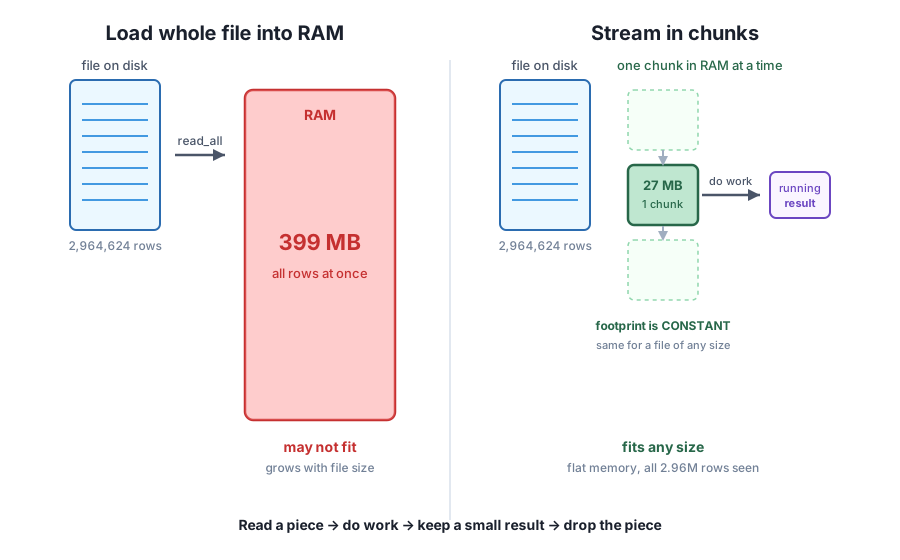
The figure contrasts the two strategies: the whole-file load builds one large block of memory that grows with the file and may not fit, while streaming slides a small fixed-size window through the file and keeps only a tiny running result.

Now Scale It Up: Streaming the Full Month with pyarrow#

The sample proved the mechanics on data that fit anyway. The real case is the full month, and here the file is parquet, not CSV. Parquet is columnar and compressed, so pd.read_csv does not apply; but the same streaming idea does, through the pyarrow library that reads parquet. A ParquetFile can report its size without loading anything, and its iter_batches method streams the file in fixed-size batches of rows — the exact parquet analogue of chunksize. The full month lives at the official TLC data URL:

# gate: skip
# The full month of trips (~50 MB parquet, 2,964,624 rows), from NYC TLC.
# Download it once, then read the local copy by name below.
import pyarrow.parquet as pq
pf = pq.ParquetFile("https://d37ci6vzurychx.cloudfront.net/trip-data/yellow_tripdata_2024-01.parquet")

With the file saved locally, open it, read its row count straight from the metadata (no data loaded), then stream every batch, convert each to a pandas DataFrame for your work, and keep only a running row count:

import warnings
warnings.filterwarnings("ignore")
import pyarrow.parquet as pq

pf = pq.ParquetFile("yellow_tripdata_2024-01.parquet")
print("rows in the full month:", f"{pf.metadata.num_rows:,}")
print("columns:", pf.metadata.num_columns)

seen = 0
peak_batch_mem = 0
for batch in pf.iter_batches(batch_size=200_000):
    df = batch.to_pandas()
    seen += len(df)
    peak_batch_mem = max(peak_batch_mem, df.memory_usage(deep=True).sum())

print(f"rows streamed:      {seen:,}")
print(f"peak batch in RAM:  {peak_batch_mem:,} bytes  ({peak_batch_mem/1024/1024:.1f} MB)")

rows in the full month: 2,964,624
columns: 19
rows streamed:      2,964,624
peak batch in RAM:  28,200,132 bytes  (26.9 MB)

This is the moment the module is built around. The running count reached 2,964,624 — you processed every row of the full month — and yet the largest amount of data ever live at once was one batch of about 27 MB. Compare that to the ~399 MB the same month would occupy loaded whole: you streamed nearly 3 million rows, data that expands well past a third of a gigabyte, while your program’s peak footprint stayed smaller than the 22.5 MB sample. Each batch is a normal pandas DataFrame after batch.to_pandas(), so everything you know still applies inside the loop. (At batch_size=200_000 the month came in 15 batches; the batch footprint is a bit larger than the CSV chunk earlier only because the parquet has 19 columns instead of 10, not because the file is bigger — it is set by batch size and column count, never by the file’s length.)

The Streaming Mindset, as a Rule#

Everything in this module is the same four-step loop, whether the source is a CSV, a parquet file, or later a database:

1. Read a piece — one chunk or batch, a bounded number of rows.
2. Do work — filter, transform, or aggregate that piece, using ordinary pandas.
3. Keep only a small result — a running count, a partial sum, a filtered handful of rows; never the pieces themselves.
4. Drop the piece — let the chunk go out of scope so its memory is freed before the next read.

The discipline lives in steps 3 and 4. The instant you start appending every chunk to a list to concatenate at the end, you have quietly rebuilt the whole-file load you were trying to avoid — all the rows end up in memory together, and the MemoryError returns. Streaming only stays flat if what you carry between iterations is genuinely small: a number, a small dictionary of group totals, a short filtered frame. Get that habit right and file size stops being a limit you fight and becomes just a count of how many loops you run.

Practice Exercises#

Exercise 1 — Prove you read every row in chunks. Load the taxi sample with pd.read_csv("yellow_tripdata_sample.csv", chunksize=25_000), loop over the iterator, count the chunks, and sum len(chunk) across them. Print the chunk count and the total, and confirm the total is 200,000 while the chunk count is 8.

Exercise 2 — Show the footprint is constant across chunk sizes. Read the sample twice, once with chunksize=20_000 and once with chunksize=80_000, tracking the peak memory_usage(deep=True).sum() of any single chunk in each pass. Print both peaks and confirm the larger chunksize has the larger peak — then explain in a comment why neither peak depends on the total file size.

Exercise 3 — Stream the parquet and count rows above a fare threshold. Open yellow_tripdata_2024-01.parquet with pyarrow.parquet.ParquetFile, stream it with iter_batches(batch_size=200_000), convert each batch with to_pandas(), and keep a single running integer: how many trips have fare_amount greater than 50. Print the running total at the end. You are computing over ~3 million rows while never holding more than one batch.

Summary#

You met the reason this module exists: loading a whole file into pandas ties peak memory to the file’s size, so a file bigger than your RAM cannot be loaded at all, no matter how aggressively you downcast it afterward. The fix is to stream. pd.read_csv(chunksize=50_000) returns a TextFileReader iterator that yields the file as real DataFrames one chunk at a time; iterating it over the 200,000-row sample gave exactly 4 chunks whose row counts summed back to 200,000 — every row processed — while the peak single chunk was 5.6 MB against the whole file’s 22.5 MB, and that 5.6 MB is set by chunksize, not by the file, so it stays constant however large the file grows. Scaling up, pyarrow’s ParquetFile.iter_batches streamed the full 2,964,624-row January parquet — data that expands to about 399 MB loaded whole — with a peak batch footprint of only ~27 MB, proving you can process nearly 3 million rows that do not comfortably fit with a tiny, flat memory footprint. The whole technique reduces to one rule: read a piece, do work, keep only a small result, drop the piece.

Key Concepts#

• Whole-file loading scales with the file — pd.read_csv("file") materializes every row at once, so peak memory grows with file size and eventually exceeds RAM; the 15 MB sample is already 22.5 MB in pandas and the full month is ~399 MB.
• pd.read_csv(chunksize=n) — returns a TextFileReader iterator, not a DataFrame; each iteration yields a real DataFrame of up to n rows. Summing len(chunk) confirms every row is processed without ever holding the whole file.
• Constant chunk footprint — a single chunk’s memory_usage(deep=True).sum() is fixed by chunksize and column count, not by the file’s length, so the same loop runs on a file of any size with the same peak memory.
• pyarrow.parquet.ParquetFile + iter_batches(batch_size=n) — the parquet analogue of chunksize; pf.metadata.num_rows reports the row count for free from the footer, and batch.to_pandas() turns each batch into an ordinary DataFrame for your work.
• The streaming rule — read a piece, do work, keep only a small result, drop the piece; accumulating the pieces themselves silently rebuilds the whole-file load you were avoiding.

Why This Matters#

Out-of-core processing is what separates a pipeline that works in a demo from one that works in production. CityFlow’s dashboard is fed by months of trip data, and no single machine holds a year of it in pandas; the only way to compute over it on ordinary hardware is to stream it, and streaming is only correct if the memory stays flat as the data grows. That flatness is the property you measured here — a constant chunk footprint independent of file size — and it is why the answer to “the data got too big” is a streaming loop, not a bigger instance you rent forever. Just as important is the mental model: once you think in pieces instead of whole files, the size of the input stops being a constraint you fear and becomes a parameter you set. Everything else in this module — streaming aggregations, incremental loads, out-of-core joins — is a variation on the loop you just wrote.

Continue Building Your Skills#

You proved you can touch every row of a file too big for RAM, but so far the “small result” you kept was only a count. The real power of streaming shows up when the result you accumulate answers a genuine analytical question. In Lesson 2, Streaming Aggregation, you will carry running sums and counts across chunks to compute statistics — like the average fare or the total tips per payment type — over data you never fully load. The trick is that a mean is just a sum divided by a count, and both a sum and a count are tiny numbers you can update chunk by chunk, so you will compute an exact average over all 2,964,624 trips while holding only two integers between iterations. That is the streaming rule from this lesson turned into a real aggregation pattern, and it is the foundation for every out-of-core computation that follows.