Lesson 2 - Streaming Aggregation

Welcome to Streaming Aggregation#

In Lesson 1 you learned to stream a file too big for RAM: pd.read_csv(chunksize=...) and pyarrow’s iter_batches hand you the data one small piece at a time, and you counted all 2,964,624 rows of the January parquet with a footprint that never grew with the file. But counting rows is the easy case. The moment CityFlow’s dashboard asks a real question — what is the average fare? — you hit a wall that looks fatal: the obvious answer is taxi["fare_amount"].mean(), and .mean() seems to need the whole column in memory at once. If you only ever hold one chunk, how can you average a column you never fully assemble?

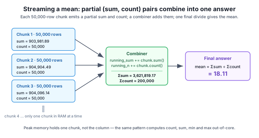
The way through is a small but powerful shift in how you think about an aggregate. A mean is not atomic. It is a ratio: total sum divided by total count. And a sum, unlike a mean, does break apart cleanly — the sum of the whole column is just the sum of each chunk’s sum. So you can walk the file chunk by chunk, add each chunk’s sum into a running total and each chunk’s count into a running count, and divide the two numbers once, at the very end. At no point do you hold more than one chunk. This lesson builds that pattern, proves it gives the exact same answer as loading the file whole, extends it to per-group aggregates, and scales it to the full month.

By the end of this lesson, you will be able to:

• Explain why a mean decomposes into a running sum and a running count, and which statistics share that property
• Stream the mean of a column with pd.read_csv(chunksize=...), accumulating sum and count per chunk
• Prove a streamed aggregate equals the whole-file result to full floating-point precision
• Build a streaming group-by by accumulating a per-group sum-and-count table with DataFrame.add(..., fill_value=0)
• Scale the streaming group-by to the full 2,964,624-row parquet with pyarrow batches and a tiny footprint
• Recognize which statistics (the median and other quantiles) do not combine across chunks, and why

You will use pandas and pyarrow. Let’s take a mean apart.

A Mean Is a Ratio, Not an Atom#

Write out the definition of an average and the whole trick falls out of it:

The numerator and denominator are the two quantities that survive being split. If you cut the column into chunks, the total sum is the sum of the chunk sums, and the total count is the sum of the chunk counts. Neither one cares about chunk boundaries. So you never need the whole column — you need two running numbers. Start by streaming just those two over the 200,000-row sample.

CityFlow’s development sample is the same 200,000-trip file you have used all course. It lives on the site here:

# gate: skip
# CityFlow's teaching sample: 200,000 real NYC yellow-taxi trips (~15 MB).
import pandas as pd
taxi = pd.read_csv("https://datatweets.com/datasets/nyc-taxi/yellow_tripdata_sample.csv")

Download it once and save it next to your script; every runnable block below reads the local copy by name. Now stream the mean fare, holding only a running total and a running n:

import warnings
warnings.filterwarnings("ignore")
import pandas as pd

total = 0.0
n = 0
for chunk in pd.read_csv("yellow_tripdata_sample.csv", chunksize=50000):
    total += chunk["fare_amount"].sum()
    n += chunk["fare_amount"].count()

streamed_mean = total / n
print(f"total fare summed: {total:,.2f}")
print(f"rows counted:      {n:,}")
print(f"streaming mean:    {streamed_mean:.10f}")

total fare summed: 3,621,819.17
rows counted:      200,000
streaming mean:    18.1090958500

The loop reads four chunks of 50,000 rows, and at no instant does it hold more than one of them. The only state that crosses a chunk boundary is two scalars — a float and an integer. total accumulated to $3,621,819.17 across all 200,000 fares, n reached exactly 200,000, and their ratio is the mean fare: $18.11. Notice the deliberate use of .count() rather than len(chunk): count() ignores missing values, so the denominator matches exactly what pandas’ own .mean() would divide by. That detail is the difference between a streamed mean that is close and one that is identical, which is what we prove next.

Proving the Stream Is Exact#

An aggregation that is approximately right is a liability — you would never know whether a reported average was off in the third decimal because of a genuine trend or because of your streaming code. So make the claim testable. Load the sample whole (you can here, because it is small) and compare pandas’ built-in mean against the streamed one:

import warnings
warnings.filterwarnings("ignore")
import pandas as pd

total = 0.0
n = 0
for chunk in pd.read_csv("yellow_tripdata_sample.csv", chunksize=50000):
    total += chunk["fare_amount"].sum()
    n += chunk["fare_amount"].count()
streamed_mean = total / n

taxi = pd.read_csv("yellow_tripdata_sample.csv")
whole_mean = taxi["fare_amount"].mean()

print(f"streaming mean:  {streamed_mean:.10f}")
print(f"whole-file mean: {whole_mean:.10f}")
print(f"difference:      {abs(streamed_mean - whole_mean):.2e}")
print(f"match within 1e-9: {abs(streamed_mean - whole_mean) < 1e-9}")

streaming mean:  18.1090958500
whole-file mean: 18.1090958500
difference:      0.00e+00
match within 1e-9: True

The difference is not merely small — it is 0.00e+00, a bit-for-bit identical result. This is the heart of the lesson: streaming a mean does not trade accuracy for memory. Because sum and count decompose exactly, and because pandas sums the chunks in the same order the whole-file mean would, you get the same floating-point answer while holding a tiny fraction of the data. The whole-file load here is only a test harness to prove correctness; in production you would delete it and keep only the loop, which runs whether the file is 200,000 rows or 200 million.

To make that concrete, carry four running values at once — sum, count, min, and max — and confirm all four match the whole-file result:

import warnings
warnings.filterwarnings("ignore")
import pandas as pd

total = 0.0
n = 0
lo = float("inf")
hi = float("-inf")
for chunk in pd.read_csv("yellow_tripdata_sample.csv", chunksize=50000):
    col = chunk["fare_amount"]
    total += col.sum()
    n += col.count()
    lo = min(lo, col.min())
    hi = max(hi, col.max())

print(f"streamed   ->  sum={total:,.2f}  count={n:,}  min={lo}  max={hi}  mean={total/n:.4f}")

whole = pd.read_csv("yellow_tripdata_sample.csv")["fare_amount"]
print(f"whole-file ->  sum={whole.sum():,.2f}  count={whole.count():,}  "
      f"min={whole.min()}  max={whole.max()}  mean={whole.mean():.4f}")

streamed   ->  sum=3,621,819.17  count=200,000  min=-700.0  max=591.7  mean=18.1091
whole-file ->  sum=3,621,819.17  count=200,000  min=-700.0  max=591.7  mean=18.1091

Every one of the four running statistics reproduces the whole-file answer exactly — including the -700.0 minimum, one of the dataset’s dirty-data oddities (a refunded or mis-keyed fare) that a real pipeline would flag. The point stands: min and max ride along in the same loop for free, because they are additive too.

Streaming a Group-By#

A single number for the whole file is useful, but CityFlow’s dashboard almost always wants a number per category — mean fare per payment type, per pickup zone, per hour. The obvious taxi.groupby("payment_type")["fare_amount"].mean() again looks like it needs the whole column. It does not, and the fix is the exact same idea, just kept per group instead of in two scalars.

For each chunk, compute a small table of sum and count per group, then add that table into a running table. The trick that makes it clean is DataFrame.add(other, fill_value=0): it adds two tables aligned by their group index, and where a group appears in one table but not the other, it treats the missing side as 0 rather than producing NaN. So a payment type that shows up only in later chunks still accumulates correctly.

import warnings
warnings.filterwarnings("ignore")
import pandas as pd

running = None
for chunk in pd.read_csv("yellow_tripdata_sample.csv", chunksize=50000):
    part = chunk.groupby("payment_type")["fare_amount"].agg(["sum", "count"])
    running = part if running is None else running.add(part, fill_value=0)

streamed = (running["sum"] / running["count"]).rename("mean_fare")
print("running per-group totals:")
print(running)
print()
print("streamed mean fare per payment_type:")
print(streamed.round(4))

running per-group totals:
                     sum   count
payment_type                    
0              189984.75    9511
1             2899332.41  156378
2              521745.22   29522
3                7225.16    1354
4                3531.63    3235

streamed mean fare per payment_type:
payment_type
0    19.9753
1    18.5405
2    17.6731
3     5.3362
4     1.0917
Name: mean_fare, dtype: float64

The running table is the whole state of the aggregation: five rows (one per payment code), two columns (sum and count), regardless of how many rows the file has. Every chunk folds its own five-row summary into it. At the end, one element-wise divide turns the totals into means: payment type 1 (credit card) averages $18.54 a fare, while type 4 (a dispute code) averages barely a dollar. Now prove the streamed table matches the answer you would get from loading everything and grouping once:

import warnings
warnings.filterwarnings("ignore")
import pandas as pd

running = None
for chunk in pd.read_csv("yellow_tripdata_sample.csv", chunksize=50000):
    part = chunk.groupby("payment_type")["fare_amount"].agg(["sum", "count"])
    running = part if running is None else running.add(part, fill_value=0)
streamed = (running["sum"] / running["count"]).rename("mean_fare")

taxi = pd.read_csv("yellow_tripdata_sample.csv")
whole = taxi.groupby("payment_type")["fare_amount"].mean().rename("mean_fare")

compare = pd.DataFrame({"streamed": streamed, "whole_file": whole})
compare["abs_diff"] = (compare["streamed"] - compare["whole_file"]).abs()
print(compare)
print()
print("max abs difference across all groups:", compare["abs_diff"].max())
print("all groups match within 1e-9:", bool((compare["abs_diff"] < 1e-9).all()))

               streamed  whole_file      abs_diff
payment_type                                     
0             19.975265   19.975265  3.552714e-15
1             18.540539   18.540539  0.000000e+00
2             17.673099   17.673099  0.000000e+00
3              5.336160    5.336160  0.000000e+00
4              1.091694    1.091694  0.000000e+00

max abs difference across all groups: 3.552713678800501e-15
all groups match within 1e-9: True

Every group matches the whole-file groupby mean. The largest discrepancy anywhere is 3.6e-15 — that is floating-point rounding at the fifteenth significant digit, the noise floor of float64 arithmetic, not a mistake in the method. For every practical purpose the streamed group-by is exact, and it held only a five-row table the entire time.

Scaling It Up to the Full Month#

The sample was small enough to check against a whole-file load. The payoff is that the identical loop works on data you cannot load whole. The January parquet is 2,964,624 rows across 19 columns — about 399 MB in pandas — but computing mean fare per payment type over all of it needs the same five-row running table you just built. Swap the CSV chunk iterator for pyarrow’s iter_batches, ask it for only the two columns you need, and stream:

import warnings
warnings.filterwarnings("ignore")
import pandas as pd
import pyarrow.parquet as pq

pf = pq.ParquetFile("yellow_tripdata_2024-01.parquet")

running = None
rows = 0
for batch in pf.iter_batches(batch_size=200_000, columns=["payment_type", "fare_amount"]):
    df = batch.to_pandas()
    rows += len(df)
    part = df.groupby("payment_type")["fare_amount"].agg(["sum", "count"])
    running = part if running is None else running.add(part, fill_value=0)

result = running.copy()
result["count"] = result["count"].astype("int64")
result["mean_fare"] = (result["sum"] / result["count"]).round(2)

print(f"rows streamed: {rows:,}")
print()
print(result[["count", "mean_fare"]])

rows streamed: 2,964,624

                count  mean_fare
payment_type                    
0              140162      20.02
1             2319046      18.56
2              439191      17.87
3               19597       6.75
4               46628       1.33

Nearly three million trips, summarized into a five-row table, while never holding more than one 200,000-row batch of two columns in memory. The columns=["payment_type", "fare_amount"] argument is doing quiet work here: parquet is columnar, so pyarrow reads only those two columns off disk and skips the other seventeen entirely, making each batch both smaller and faster. The result is CityFlow’s real answer for January: credit-card fares (type 1) average $18.56 across 2.3 million rides, and every payment code’s mean is computed over the full month with a footprint measured in tens of megabytes, not hundreds.

import warnings
warnings.filterwarnings("ignore")
import pandas as pd

fares = pd.read_csv("yellow_tripdata_sample.csv")["fare_amount"]
true_median = fares.median()

# Real streams often arrive already ordered (by time, by id). Simulate that
# worst case by sorting, then walk it in 50,000-row chunks.
ordered = fares.sort_values().reset_index(drop=True)
chunk_medians = [ordered.iloc[i:i + 50000].median() for i in range(0, len(ordered), 50000)]

naive = sum(chunk_medians) / len(chunk_medians)
print("per-chunk medians:", [round(float(m), 2) for m in chunk_medians])
print(f"average of chunk medians: {naive:.4f}")
print(f"true median (whole file): {true_median:.4f}")
print(f"they disagree: {naive != true_median}")

per-chunk medians: [6.83, 10.7, 15.6, 32.72]
average of chunk medians: 16.4625
true median (whole file): 12.8000
they disagree: True

Practice Exercises#

Exercise 1 — Stream a mean and prove it exact. Stream the mean of total_amount over yellow_tripdata_sample.csv using pd.read_csv(chunksize=50000), accumulating a running sum and a running count. Then load the file whole, compute taxi["total_amount"].mean(), and print both values plus their absolute difference. Confirm the difference is below 1e-9.

Exercise 2 — Stream a group-by over the sample. Compute the mean tip_amount per payment_type by streaming the sample: for each chunk build chunk.groupby("payment_type")["tip_amount"].agg(["sum", "count"]) and fold it into a running table with .add(..., fill_value=0). Divide sum by count at the end, then verify your result matches taxi.groupby("payment_type")["tip_amount"].mean() on a whole-file load.

Exercise 3 — Scale the group-by to the full month. Stream yellow_tripdata_2024-01.parquet with pq.ParquetFile(...).iter_batches(batch_size=200_000, columns=[...]), requesting only the columns you need, and compute the mean trip_distance per passenger_count over all 2,964,624 rows. Print the total rows streamed and the resulting per-group means, and note how much smaller your running table is than the file.

Summary#

You turned a stream of chunks into a single exact answer. The key realization is that a mean is not atomic — it is total_sum / total_count — so you can accumulate a running sum and a running count chunk by chunk and divide once at the end, holding only two scalars. Streaming the mean fare over the 200,000-row sample gave $18.11, and comparing it to taxi["fare_amount"].mean() produced a difference of exactly 0.00e+00: streaming buys memory without costing accuracy. The same decomposition covers sum, count, min, and max (all additive statistics), and it extends to a group-by by accumulating a small per-group sum-and-count table with DataFrame.add(..., fill_value=0) — which matched the whole-file groupby mean to within floating-point noise. Finally the identical loop scaled to the full 2,964,624-row January parquet through pyarrow’s iter_batches, computing mean fare per payment type over three million rows with a five-row running table. The honest boundary: the median and other quantiles are order statistics that do not decompose this way, so exact streaming stops at additive aggregates.

Key Concepts#

• A mean is a ratio — total_sum / total_count, so both the numerator and denominator decompose across chunks; accumulate a running sum and count, and divide once at the end.
• Additive statistics stream — sum, count, min, and max each need one running scalar; the mean needs two, the variance three. Use .count() (not len) so the denominator excludes missing values exactly as pandas does.
• Prove exactness — compare the streamed result against a whole-file .mean()/.groupby().mean() on a sample small enough to load; a 0-to-1e-15 difference confirms the method before you trust it on data you cannot load whole.
• Streaming group-by — per chunk, compute groupby(...)["col"].agg(["sum", "count"]); fold it into a running table with DataFrame.add(other, fill_value=0); divide sum by count at the end. The running state is one row per group, independent of file size.
• Order statistics do not stream — the median and percentiles depend on the global ordering of every value; per-chunk summaries cannot recover them exactly. Use a t-digest or reservoir sample to approximate them in one pass.

Why This Matters#

Almost every metric on CityFlow’s dashboard — average fare, total revenue, trips per zone, mean tip by payment type — is an additive aggregate, which means the streaming pattern in this lesson is not a niche trick but the everyday engine of out-of-core reporting. It lets a modest worker summarize a month, a quarter, or a year of trips with a memory footprint that depends on the number of groups, not the number of rows, and it does so without giving up a single digit of accuracy versus loading the data whole. Just as important is the discipline you practiced: prove the streamed answer equals the whole-file answer on a sample first, so that when you run the loop on data too big to check, you already trust it. And knowing the boundary — that a median needs a different tool — is exactly the kind of judgment that separates a pipeline that quietly reports wrong numbers from one an analyst can rely on.

Continue Building Your Skills#

Streaming an aggregate is perfect when you need one summary from one pass over the data. But notice what happens the second time CityFlow asks a question: if next you want mean fare per pickup zone, or trips per hour, or revenue per day, you have to stream the entire multi-hundred-megabyte file all over again from scratch. Re-reading three million rows for every new question gets expensive fast. In Lesson 3, SQLite as a Local Warehouse, you will break that cycle by streaming the chunks once into an on-disk SQLite database with the standard-library sqlite3 module — persisting the data into a queryable store so that every later question is a fast SELECT ... GROUP BY against an indexed table instead of another full re-stream. You will keep the exact same chunked-reading habit from this module, but point it at a durable warehouse instead of a throwaway running total.