Title here
Summary here
In Lesson 2 you learned to stream the full month of trips through pandas in chunks, computing a result without ever holding all 2.96 million rows in memory at once. That technique is exactly right for a one-pass job. But look at what it costs when CityFlow’s dashboard needs five different numbers from the same month: each one re-opens the 50 MB parquet file, re-decodes every batch, and re-streams all 2,964,624 rows from scratch. You pay the full read five times to answer five questions. Streaming has no memory between runs.
This lesson fixes that with a better pattern for repeated queries: stream the data in once, into a real database on disk, then query it as many times as you like. The database is SQLite — a genuine, serverless, file-based SQL engine that ships inside Python’s standard library as the sqlite3 module. There is nothing to install and no server to start; a database is just a file. You will stream the month into a trips table where the rows live on disk, then run ordinary SQL — GROUP BY, WHERE, and indexes — over all 3 million of them while only ever pulling tiny results back into pandas. That is out-of-core querying: the data stays on disk, and only the answer comes to you.
By the end of this lesson, you will be able to:
pyarrow batches and df.to_sql(..., if_exists="append")SELECT COUNT(*) and measure the database file’s real size on diskGROUP BY aggregation that scans ~3M rows and returns a handfulCREATE INDEX, read EXPLAIN QUERY PLAN, and measure the speedup a selective query getsYou only need pandas, pyarrow, and the stdlib sqlite3. Let’s build a warehouse.
Streaming is stateless by design, and that is both its strength and its weakness. A chunked pass holds almost no memory, but it also remembers nothing: the moment it finishes, the parsed rows are gone, and the next question starts the whole read over. For a pipeline that runs a single aggregation nightly, that is fine. For an interactive dashboard, or any workflow that asks many questions of the same data, re-decoding a 50 MB parquet into ~3 million rows for every query is pure waste.
A local database flips the trade. You pay the streaming cost once to load the rows into a file on disk, and from then on every query reads that file with the database engine’s own machinery — which is written in C, understands your data’s layout, and can use indexes to skip rows it does not need. SQLite is the perfect tool for this at laptop scale: the entire database is one ordinary file you can copy, back up, or delete; it needs no running server; and it speaks standard SQL. The rows sit on disk, not in RAM, so the size of your data is bounded by your disk, not your memory — the whole point of this module.
CityFlow’s full month lives in the official public parquet file. You would download it once:
# gate: skip
# The real January 2024 month, straight from the NYC TLC (~50 MB, 2,964,624 rows).
import pyarrow.parquet as pq
url = "https://d37ci6vzurychx.cloudfront.net/trip-data/yellow_tripdata_2024-01.parquet"
pf = pq.ParquetFile(url)   # download once, then read the local copy by name
Save that file next to your script as yellow_tripdata_2024-01.parquet; every runnable block below reads the local copy by name.
The load is a marriage of two techniques you already know. You stream the parquet in batches with pyarrow (so the whole file never sits in memory), and you append each batch to a database table with pandas’ to_sql. A sqlite3 connection is just sqlite3.connect("warehouse.db") — if the file does not exist, SQLite creates it. Because we want the lesson to be repeatable, the very first thing we do is delete any leftover database from a previous run, so we always start clean.
We keep a useful subset of the 19 parquet columns — the pickup time, the two zone IDs, and the money and count columns — and pass that list straight to iter_batches so pyarrow only reads what we need. Each 200,000-row batch becomes a small DataFrame that we append to the trips table; the first to_sql call creates the table from the DataFrame’s columns, and every later call adds rows to it.
import warnings
warnings.filterwarnings("ignore")
import os, sqlite3
import pandas as pd
import pyarrow.parquet as pq

# Idempotent: start from a clean database file every run.
os.path.exists("warehouse.db") and os.remove("warehouse.db")

keep = ["tpep_pickup_datetime", "PULocationID", "DOLocationID",
        "passenger_count", "trip_distance", "fare_amount",
        "tip_amount", "total_amount"]

con = sqlite3.connect("warehouse.db")
trips_file = pq.ParquetFile("yellow_tripdata_2024-01.parquet")

batches = 0
for batch in trips_file.iter_batches(batch_size=200_000, columns=keep):
    frame = batch.to_pandas()
    frame["tpep_pickup_datetime"] = frame["tpep_pickup_datetime"].astype(str)
    frame.to_sql("trips", con, if_exists="append", index=False)
    batches += 1

rows = pd.read_sql("SELECT COUNT(*) AS n FROM trips", con)["n"].iloc[0]
size_mb = os.path.getsize("warehouse.db") / 1024 / 1024
print(f"batches appended : {batches}")
print(f"rows in trips    : {rows:,}")
print(f"warehouse.db size: {size_mb:.1f} MB on disk")
con.close()
batches appended : 15
rows in trips : 2,964,624
warehouse.db size: 186.4 MB on diskThe whole month streamed through in 15 batches of 200,000 rows, and SELECT COUNT(*) confirms every one of the 2,964,624 trips landed in the table. At no point did all three million rows share memory — the largest DataFrame alive was a single 200,000-row batch. The result is a 186.4 MB file called warehouse.db sitting on your disk. That file is larger than the 50 MB parquet (parquet is compressed and columnar; SQLite stores plain rows plus its own bookkeeping), but it is far smaller than the ~400 MB the same data costs as a live pandas DataFrame — and, crucially, it is on disk, ready to answer questions without being rebuilt.
One small detail earns its keep: we cast tpep_pickup_datetime to a string before inserting. SQLite has no native datetime type — it stores dates as text or numbers — and passing the timestamps as ISO-formatted strings ("2024-01-15 09:32:00") keeps them sortable and comparable in SQL. It is the honest, portable choice for a stdlib SQLite table.
to_sql needs the whole frame in memory — so feed it batches
df.to_sql inserts every row of the DataFrame you hand it, so calling it once on a 3-million-row frame would defeat the entire purpose — you would have loaded the whole month into RAM first. The pattern that stays out-of-core is exactly the one above: stream small batches with iter_batches, and call to_sql(..., if_exists="append") once per batch. Each call only holds 200,000 rows. The database file on disk grows; your memory footprint does not.
Now the payoff. The month is on disk, and you never have to stream it again — you just ask SQL questions. Which taxi zones start the most trips? That is a GROUP BY over all 2.96 million rows, and SQLite does the entire scan-and-aggregate inside its C engine, handing pandas back only the finished ten-row answer:
import warnings
warnings.filterwarnings("ignore")
import sqlite3
import pandas as pd

con = sqlite3.connect("warehouse.db")
busiest = pd.read_sql(
    "SELECT PULocationID, COUNT(*) trips, AVG(fare_amount) avg_fare "
    "FROM trips "
    "GROUP BY PULocationID "
    "ORDER BY trips DESC "
    "LIMIT 10", con)
con.close()
print(busiest.round(2).to_string(index=False))
PULocationID trips avg_fare
132 145240 59.40
161 143471 15.21
237 142708 12.18
236 136465 12.71
162 106717 14.79
230 106324 17.54
186 104523 15.79
142 104080 13.43
138 89533 41.46
239 88474 13.45This is out-of-core aggregation in one line of SQL. SQLite walked all 2,964,624 rows on disk, counted and averaged them by zone, sorted the groups, and returned the top ten — a DataFrame of ten rows. The full three million rows never entered pandas. Only the tiny result did. Compare that to the streaming approach from Lesson 2, where you had to write the chunk loop, maintain running totals across batches, and combine them at the end. Here the database engine does all of it, and you express the whole computation declaratively.
The numbers themselves are a nice sanity check on the data. Zone 132 is JFK Airport, and its telltale avg_fare of $59.40 (airport trips are long and often flat-rated) stands out against the ~$12–17 fares of the dense-Manhattan zones like 161, 237, and 236 that follow it. Zone 138 (LaGuardia) shows the same airport signature at $41.46. The SQL result is not just fast — it is telling you something true about the city.
The GROUP BY above had to visit every row, so a full scan of the table is unavoidable — and 3 million rows on disk is genuinely fast in SQLite. But many dashboard queries are selective: they ask about one zone, one day, one payment type. For those, scanning all 3 million rows to find the few thousand that match is wasteful, and this is exactly what an index fixes. An index is a sorted, on-disk lookup structure on a column; with one in place, SQLite can jump straight to the matching rows instead of reading the whole table.
You can see the difference before you even time it, using EXPLAIN QUERY PLAN — SQLite tells you how it intends to run a query. Let’s take a filtered lookup on the busiest zone, check the plan and time it, then add an index and do it again. Note that we drop the index first so the block is repeatable:
import warnings
warnings.filterwarnings("ignore")
import sqlite3, time
import pandas as pd

con = sqlite3.connect("warehouse.db")
con.execute("DROP INDEX IF EXISTS idx_pu")   # start from a clean, unindexed table

busy = ("SELECT COUNT(*) trips, AVG(total_amount) avg_total "
        "FROM trips WHERE PULocationID = 132")

def elapsed_ms(sql):
    start = time.perf_counter()
    pd.read_sql(sql, con)
    return (time.perf_counter() - start) * 1000

plan_before = pd.read_sql("EXPLAIN QUERY PLAN " + busy, con)["detail"].iloc[0]
t_before = elapsed_ms(busy)

con.execute("CREATE INDEX idx_pu ON trips(PULocationID)")

plan_after = pd.read_sql("EXPLAIN QUERY PLAN " + busy, con)["detail"].iloc[0]
t_after = elapsed_ms(busy)

print(f"before -> plan: {plan_before}")
print(f"before -> time: {t_before:.0f} ms")
print(f"after  -> plan: {plan_after}")
print(f"after  -> time: {t_after:.0f} ms")
print(f"speedup: {t_before / t_after:.1f}x")
con.close()
before -> plan: SCAN trips
before -> time: 146 ms
after -> plan: SEARCH trips USING INDEX idx_pu (PULocationID=?)
after -> time: 86 ms
speedup: 1.7xThe query plan is the story. Before the index, SQLite reports SCAN trips — it reads every row to find the matches. After CREATE INDEX idx_pu ON trips(PULocationID), the same query plans as SEARCH trips USING INDEX idx_pu — it now uses the sorted structure to seek. The wall-clock time dropped from about 146 ms to 86 ms, a 1.7× speedup. (These timings shift run to run — disk cache, other processes, and warm-up all nudge them by tens of milliseconds — so treat the ratio as the signal, not the exact numbers.)
A 1.7× win is real but modest, and the reason is instructive: zone 132 is the single busiest zone in the city, matching 145,240 rows — about 5% of the whole table. Even with the index, SQLite still has to read all 145,240 of them, so the index saves the scan of the other 95% but not much more. The index pays off far more dramatically when a query is selective — when only a handful of rows match.
Zone 12 (Battery Park) is a quiet zone with only a few hundred pickups all month. That is where the index earns its keep. Watch the same query shape against a selective filter, timed with no index and then with one:
import warnings
warnings.filterwarnings("ignore")
import sqlite3, time
import pandas as pd

con = sqlite3.connect("warehouse.db")
con.execute("DROP INDEX IF EXISTS idx_pu")

selective = ("SELECT COUNT(*) trips, AVG(total_amount) avg_total "
             "FROM trips WHERE PULocationID = 12")

def elapsed_ms(sql):
    start = time.perf_counter()
    result = pd.read_sql(sql, con)
    return result, (time.perf_counter() - start) * 1000

res_before, t_before = elapsed_ms(selective)      # full scan
con.execute("CREATE INDEX idx_pu ON trips(PULocationID)")
res_after, t_after = elapsed_ms(selective)        # index seek

print(res_after.round(2).to_string(index=False))
print(f"full scan  : {t_before:.0f} ms")
print(f"indexed    : {t_after:.1f} ms")
print(f"speedup    : {t_before / t_after:.0f}x")
con.close()
trips avg_total
875 31.22
full scan : 163 ms
indexed : 2.2 ms
speedup : 75xZone 12 matched only 875 rows out of 2.96 million. Without the index, SQLite still had to scan the whole table to find them — about 163 ms, the same cost as any full scan. With the index, it seeks straight to those 875 rows in roughly 2 ms, a 75× speedup. This is the general rule of thumb: an index helps in proportion to how few rows a query keeps. A filter that returns 5% of the table gets a small boost; a filter that returns a fraction of a percent gets an enormous one. Index the columns you filter and join on, and your selective dashboard queries stop scanning millions of rows they were only going to throw away.
The figure below traces the whole pattern: stream the month in once, keep the rows on disk, then let SQL pull tiny results out — a ten-row aggregate from a full scan, or a handful of rows from an indexed search.
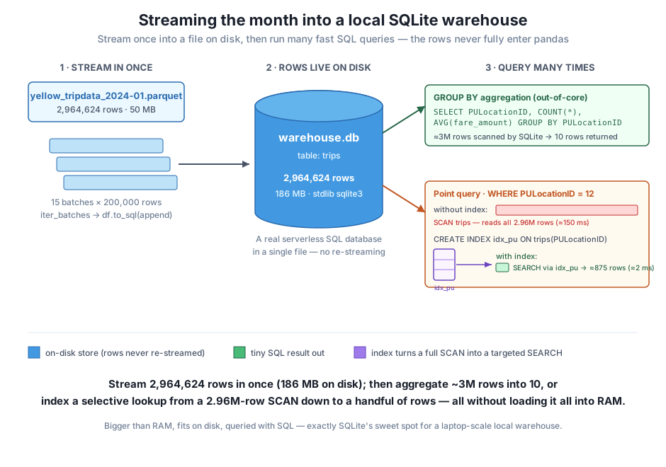
warehouse.db once (15 batches of 200,000 rows, 186 MB on disk) so the 2,964,624 trips live on disk rather than in RAM. Then query many times: a single GROUP BY scans ~3M rows and returns just 10, and a selective WHERE lookup drops from a full SCAN (≈150 ms) to a targeted SEARCH via idx_pu (≈2 ms) once an index exists — all without loading the whole table into pandas. This is SQLite's sweet spot: bigger than RAM, fits on disk, queried with SQL.SQLite is a local warehouse, not a distributed one
SQLite is exactly right for a laptop-scale warehouse: data measured in gigabytes, sitting in one file, queried with SQL, by a single writer at a time. It is serverless, zero-configuration, and rock-solid — a superb fit for “bigger than RAM, fits on disk.” What it is not is a distributed system: it does not spread data across a cluster of machines or handle many concurrent writers, and it will not crunch terabytes across dozens of nodes. That job belongs to engines like Apache Spark, which a later course covers. Reach for SQLite when your data outgrows RAM but still fits comfortably on one disk — which, for a great many real pipelines, it does.
Exercise 1 — Build the warehouse and verify the load. Stream yellow_tripdata_2024-01.parquet into a fresh warehouse.db using iter_batches and df.to_sql(..., if_exists="append"), keeping the eight columns from the lesson. Remove any existing warehouse.db first so the load is idempotent. Then confirm with a single SELECT COUNT(*) that the table holds 2,964,624 rows, and print the file’s size on disk with os.path.getsize.
Hint
Open the connection with sqlite3.connect("warehouse.db"). Loop for batch in pq.ParquetFile("yellow_tripdata_2024-01.parquet").iter_batches(batch_size=200_000, columns=keep):, call batch.to_pandas(), cast tpep_pickup_datetime to str, and frame.to_sql("trips", con, if_exists="append", index=False). Read the count back with pd.read_sql("SELECT COUNT(*) AS n FROM trips", con) and the size with os.path.getsize("warehouse.db") / 1024 / 1024.
Exercise 2 — Ask a new question with SQL, not a chunk loop. Against the warehouse.db you built, write one pd.read_sql query that returns, for each passenger_count, the number of trips and the average total_amount, ordered by trip count descending. You are aggregating ~3M on-disk rows into a few rows — note in a comment how many rows come back into pandas versus how many SQLite scanned.
Hint
The query is SELECT passenger_count, COUNT(*) trips, AVG(total_amount) avg_total FROM trips GROUP BY passenger_count ORDER BY trips DESC. It returns one row per distinct passenger count (a handful), even though SQLite scanned all 2,964,624 rows to build it. That gap — millions scanned, a few returned — is the out-of-core aggregation you are practicing.
Exercise 3 — Prove an index helps a selective join column. Dashboard queries also filter on the drop-off zone DOLocationID. Pick a selective zone (one with few trips), time a SELECT COUNT(*) ... WHERE DOLocationID = <that zone> query with time.perf_counter(), then CREATE INDEX idx_do ON trips(DOLocationID), run the same query again, and report the two timings and their ratio. Confirm with EXPLAIN QUERY PLAN that the plan changes from SCAN trips to SEARCH trips USING INDEX idx_do.
Hint
Find a quiet zone first with SELECT DOLocationID, COUNT(*) n FROM trips GROUP BY DOLocationID ORDER BY n ASC LIMIT 10. Wrap pd.read_sql between two time.perf_counter() calls for the timing, and remember to DROP INDEX IF EXISTS idx_do at the start if you want the block to be re-runnable. The more selective the zone, the larger the speedup you will measure — just as zone 12 beat zone 132 in the lesson.
You replaced “re-stream the file for every question” with “stream once, query forever.” Using only Python’s standard library, you connected to a SQLite database — a real, serverless, file-based SQL engine — and streamed the full January month into it with pyarrow’s iter_batches feeding pandas’ df.to_sql(..., if_exists="append") one 200,000-row batch at a time, so the whole table never touched RAM. SELECT COUNT(*) verified all 2,964,624 rows landed, in a 186.4 MB file on disk. From there you queried out-of-core: a single GROUP BY scanned ~3 million on-disk rows and returned just ten, the full table never entering pandas. Then you met indexes: EXPLAIN QUERY PLAN showed a query change from SCAN trips to SEARCH trips USING INDEX idx_pu, and timing showed why selectivity matters — the busiest zone (145,240 rows) sped up only ~1.7×, while a selective zone (875 rows) dropped from ~163 ms to ~2 ms, a ~75× win.
to_sql — df.to_sql inserts the whole frame it is given, so stay out-of-core by feeding it iter_batches batches and using if_exists="append"; the first call creates the table, later calls add rows.GROUP BY runs entirely inside SQLite over the on-disk rows and returns only the small result to pandas; the millions of rows never load into memory.EXPLAIN QUERY PLAN — CREATE INDEX builds a sorted on-disk lookup so a filter plans as SEARCH ... USING INDEX instead of SCAN; the plan tells you which one you get before you time it.For CityFlow, this is the difference between a dashboard that re-decodes 50 MB of parquet on every click and one that answers in milliseconds from a file it built once. A local SQLite warehouse gives a data engineer a genuine SQL layer with no infrastructure to run — you can back it up by copying a file, ship it alongside a repo, and query it from any language that speaks SQLite. Just as important is the mental model you practiced: keep the data on disk, push the computation down into the engine, and pull back only the small result. That is the same principle that scales all the way up to distributed warehouses — you are simply learning it on the version that fits on your laptop. And because the database persists, the natural next question is how to grow it over time without rebuilding it from scratch.
Your warehouse.db holds January, but CityFlow’s data does not stop at one month — February arrives, then March, and re-streaming the entire history every time a new file lands would throw away the very savings you just built. In Lesson 4, Incremental & Resumable Pipelines, you will make the warehouse grow: appending next month’s trips to the existing table without reprocessing the months already loaded, and designing the load so that re-running it is safe — idempotent — rather than silently doubling your rows. You will track what has already been ingested, skip what is done, and resume cleanly after an interruption, turning today’s one-shot loader into a pipeline you can run every day.
Keep DATATWEETS free. Help fund practical data, AI, and engineering lessons for learners worldwide.

