Lesson 5 - Guided Project: Aggregate Months That Don't Fit

Welcome to the Guided Project#

Across this module you took apart the assumption that your data has to fit in memory. You streamed a file in bounded chunks so the footprint never grew, you accumulated sums and counts across chunks to compute results over data you never fully held, you loaded chunks into a local SQLite warehouse you could query with real SQL and indexes, and you made a pipeline incremental and resumable with a ledger so re-running it was safe and cheap. Each of those was a single technique on its own dataset. This project is where they become one pipeline.

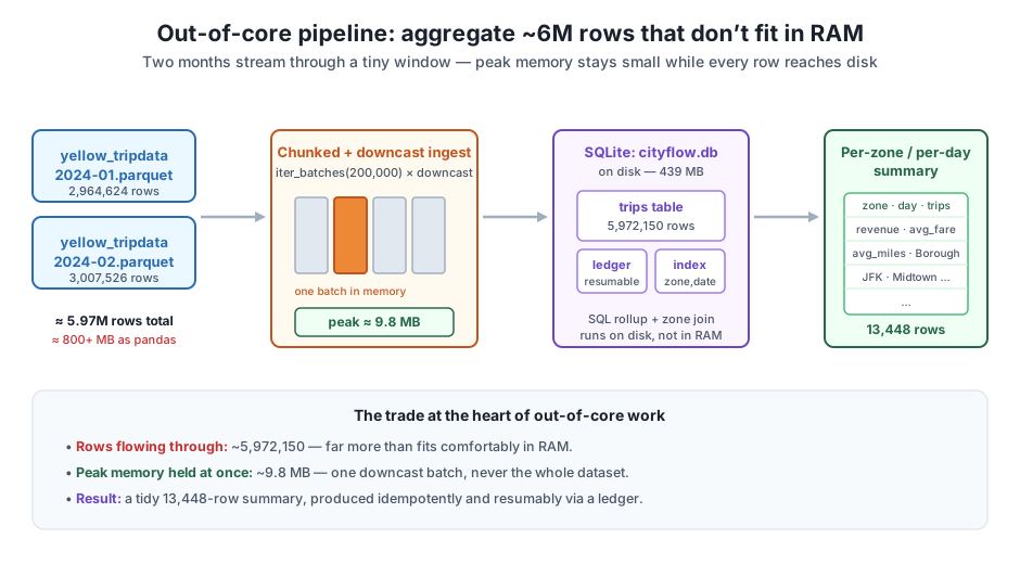
You are a data engineer at CityFlow, and the dashboard team wants a per-zone, per-day summary of taxi activity — trips, revenue, average fare, average distance — for a two-month window. The catch is the scale. One month of NYC yellow taxi trips is nearly three million rows; two months together is 5,972,150 rows, which lands around 800 MB or more as a naive pandas DataFrame. You are not going to load that. Instead you will stream both months through a tiny window, land them on disk, and let SQL do the aggregation where the data already lives.

The deliverable is a single, re-runnable script that ingests more data than fits comfortably in RAM and hands back a small, tidy summary — the kind of table a dashboard can read in a blink. Every number below is measured on the real files, and you will reproduce every one of them.

By the end of this project, you will be able to:

• Stream multiple month-sized Parquet files with a peak memory footprint of a few tens of megabytes
• Downcast each batch on the way in so the on-disk warehouse stays lean
• Make the ingest idempotent and resumable with a loaded_months ledger
• Index and roll up millions of rows into a compact per-zone, per-day summary with one SQL query
• Join the summary to real borough and zone names, and handle genuine dirty data honestly

The dataset#

Everything runs on New York City’s public-domain Yellow Taxi trip records, published by the NYC Taxi & Limousine Commission (TLC). This project uses two full months — the official TLC Parquet files — because the whole point is to process more data than fits in memory at once:

• January 2024, 2,964,624 rows: https://d37ci6vzurychx.cloudfront.net/trip-data/yellow_tripdata_2024-01.parquet
• February 2024, 3,007,526 rows: https://d37ci6vzurychx.cloudfront.net/trip-data/yellow_tripdata_2024-02.parquet

To attach human-readable names, you also use the small zone lookup dimension (265 zones, mapping each LocationID to a borough and zone name), which you met earlier in the course:

• Zone lookup (4 columns): https://datatweets.com/datasets/nyc-taxi/taxi_zone_lookup.csv

In a real pipeline you download each month once from its public URL and then read the local cached copy — the code below reads the bare local filenames, exactly as the pipeline does after caching:

# gate: skip
# The real public source: one Parquet file per month on the TLC CloudFront host.
BASE = "https://d37ci6vzurychx.cloudfront.net/trip-data/"
for month in ("2024-01", "2024-02"):
    print(BASE + f"yellow_tripdata_{month}.parquet")

Stage 1: Setup and config#

A good pipeline starts by naming exactly what it will process and making itself safe to run twice. You list the months to load with their local filenames, and — because a re-run should never double-count rows or trip over a half-built database — you delete any previous cityflow.db at the very start. That one line is what makes the whole project idempotent: run it once or run it ten times, and you end with the same clean result.

import warnings
warnings.filterwarnings("ignore")
import os, sqlite3
import pandas as pd
import pyarrow.parquet as pq

DB = "cityflow.db"
if os.path.exists(DB):
    os.remove(DB)          # start clean so the whole project re-runs cleanly

MONTHS = {
    "2024-01": "yellow_tripdata_2024-01.parquet",
    "2024-02": "yellow_tripdata_2024-02.parquet",
}

for month, fname in MONTHS.items():
    print(f"{month}  ->  {fname}")
print("combined scale: ~2.96M + ~3.01M = ~5.97M rows (far more than fits comfortably in RAM)")

2024-01  ->  yellow_tripdata_2024-01.parquet
2024-02  ->  yellow_tripdata_2024-02.parquet
combined scale: ~2.96M + ~3.01M = ~5.97M rows (far more than fits comfortably in RAM)

The plan is set: two months, roughly six million rows combined. Held all at once in pandas, that is well over half a gigabyte — so the ingest that comes next never loads a whole month at a time. It reads each file in batches, shrinks each batch, writes it to disk, and throws it away.

Stage 2: Chunked, downcast ingest with a ledger#

This is the heart of the project, and it folds three techniques from the module into one function. From Lesson 1, you stream each month with pq.ParquetFile(path).iter_batches(...) so only one batch is ever in memory. From Module 3, you downcast the numeric columns of each batch before writing, so the copy that lands in SQLite is as small as the copy in memory. From Lesson 4, you keep a ledger — a loaded_months table — so a month that is already loaded is skipped instead of appended a second time.

load_month does all of it. For each batch it selects only the columns the summary needs, derives a text pickup_date (so you can group and filter by calendar day with plain string comparisons), tags the row with its month, downcasts the numerics, and appends to the trips table. It also tracks a running peak — the largest single batch’s deep memory — because that peak, not the total, is the true memory cost of the whole job.

KEEP = ["tpep_pickup_datetime", "PULocationID",
        "trip_distance", "fare_amount", "total_amount"]

con = sqlite3.connect(DB)
con.execute("CREATE TABLE IF NOT EXISTS loaded_months (month TEXT PRIMARY KEY)")
con.commit()

def already_loaded(con, month):
    return con.execute(
        "SELECT 1 FROM loaded_months WHERE month = ?", (month,)
    ).fetchone() is not None

def load_month(con, month, path, batch_size=200_000):
    """Stream one month's parquet in batches, downcast, append to `trips`.
    Idempotent: a month already in the ledger is skipped."""
    if already_loaded(con, month):
        print(f"{month}: already in ledger - skipping")
        return 0, 0
    rows, peak = 0, 0
    pf = pq.ParquetFile(path)
    for batch in pf.iter_batches(batch_size=batch_size, columns=KEEP):
        df = batch.to_pandas()
        # derive a text pickup_date + a month tag, drop the raw timestamp
        df["pickup_date"] = pd.to_datetime(df["tpep_pickup_datetime"]).dt.date.astype(str)
        df["month"] = month
        df = df.drop(columns=["tpep_pickup_datetime"])
        # downcast numerics (Module 3) so each batch is as small as possible
        df["PULocationID"] = pd.to_numeric(df["PULocationID"], downcast="integer")
        for col in ["trip_distance", "fare_amount", "total_amount"]:
            df[col] = pd.to_numeric(df[col], downcast="float")
        peak = max(peak, int(df.memory_usage(deep=True).sum()))
        df.to_sql("trips", con, if_exists="append", index=False)
        rows += len(df)
    con.execute("INSERT INTO loaded_months (month) VALUES (?)", (month,))
    con.commit()
    print(f"{month}: {rows:,} rows appended  (peak batch {peak/1024**2:.1f} MB)")
    return rows, peak

total_rows, peak_bytes = 0, 0
for month, fname in MONTHS.items():
    n, p = load_month(con, month, fname)
    total_rows += n
    peak_bytes = max(peak_bytes, p)

print(f"\ntotal rows processed:  {total_rows:,}")
print(f"peak per-batch memory: {peak_bytes/1024**2:.1f} MB")
print("ledger:", con.execute("SELECT month FROM loaded_months ORDER BY month").fetchall())

2024-01: 2,964,624 rows appended  (peak batch 9.0 MB)
2024-02: 3,007,526 rows appended  (peak batch 9.8 MB)

total rows processed:  5,972,150
peak per-batch memory: 9.8 MB
ledger: [('2024-01',), ('2024-02',)]

There is the whole promise of out-of-core processing on one line: 5,972,150 rows processed, 9.8 MB held at the peak. The pipeline moved nearly six million rows — more than would fit comfortably in memory as a single DataFrame — while never holding more than one downcast batch of 200,000 rows at a time. The footprint is set by the batch size and the column count, not by the size of the dataset, so a third month or a tenth would not raise that 9.8 MB at all. The ledger now records both months, which is what makes the next block interesting.

Because the ledger is checked before any reading happens, re-running a month is a no-op. Call load_month again for January and it returns immediately, without touching the file or the trips table:

load_month(con, "2024-01", MONTHS["2024-01"])

2024-01: already in ledger - skipping

That is the resumability you built in Lesson 4, now protecting a real ingest. If the script crashed halfway through February and you restarted it, January would be skipped and only the missing month would load. Re-running the whole pipeline is always safe.

Stage 3: Index the group-by columns#

The summary groups every row by pickup zone and pickup day, so those are the columns SQLite should be able to find quickly. A composite index on (PULocationID, pickup_date) lets the database organize its scan around exactly the grouping the rollup asks for, instead of walking all 5.97 million rows blindly. You build the index once, after the data is loaded, and every query that groups on those columns benefits.

con.execute("CREATE INDEX IF NOT EXISTS idx_zone_date ON trips(PULocationID, pickup_date)")
con.commit()

idx = con.execute(
    "SELECT name FROM sqlite_master WHERE type='index' AND tbl_name='trips'"
).fetchall()
print("indexes on trips:", idx)

indexes on trips: [('idx_zone_date',)]

The index is in place. It costs a little disk space and a moment to build, but it is the difference between a rollup that scans the table thoughtfully and one that grinds through every row — exactly the trade you make in any warehouse when you know which columns you will group and filter on.

Stage 4: The rollup#

Now the payoff. A single GROUP BY query turns the ~6 million individual trips into one row per zone per day, carrying the four measures the dashboard wants: a trip count, total revenue, average fare, and average distance. This runs inside SQLite, over the data on disk — pandas never holds the six million rows to compute it. What comes back is small enough to fit in memory with room to spare.

ROLLUP = """
SELECT PULocationID,
       pickup_date,
       COUNT(*)                    AS trips,
       ROUND(SUM(total_amount),2)  AS revenue,
       ROUND(AVG(fare_amount),2)   AS avg_fare,
       ROUND(AVG(trip_distance),2) AS avg_miles
FROM trips
GROUP BY PULocationID, pickup_date
"""
summary = pd.read_sql(ROLLUP, con)
print("summary shape:", summary.shape)

summary shape: (13466, 6)

Six million rows in, 13,466 rows out — a summary roughly 440 times smaller than the raw data, and the whole reason the pipeline exists. A dashboard cannot page through six million trips, but 13,466 zone-days is a table it can load, chart, and filter instantly.

Those rows still speak in numeric zone IDs, though. To make the summary readable you join it to the taxi_zone_lookup.csv dimension, which maps each LocationID to its borough and zone name. Load the lookup into its own table, then join and ask a concrete question: on a representative in-month day, January 15th, which pickup zones brought in the most revenue?

zones = pd.read_csv("taxi_zone_lookup.csv")
zones.to_sql("zones", con, if_exists="replace", index=False)

top_day = pd.read_sql("""
    SELECT s.PULocationID, z.Borough, z.Zone,
           s.trips, s.revenue, s.avg_fare, s.avg_miles
    FROM ( SELECT PULocationID,
                  COUNT(*)                    AS trips,
                  ROUND(SUM(total_amount),2)  AS revenue,
                  ROUND(AVG(fare_amount),2)   AS avg_fare,
                  ROUND(AVG(trip_distance),2) AS avg_miles
           FROM trips
           WHERE pickup_date = '2024-01-15'
           GROUP BY PULocationID ) s
    JOIN zones z ON z.LocationID = s.PULocationID
    ORDER BY s.revenue DESC
    LIMIT 8
""", con)
print(top_day.to_string(index=False))

 PULocationID   Borough                         Zone  trips   revenue  avg_fare  avg_miles
          132    Queens                  JFK Airport   5651 445988.31     61.17      15.97
          138    Queens            LaGuardia Airport   3497 216302.71     39.35       9.36
          161 Manhattan               Midtown Center   3330  78485.11     15.62       2.64
          230 Manhattan    Times Sq/Theatre District   2916  77639.83     17.73       3.16
          186 Manhattan Penn Station/Madison Sq West   3367  76033.58     15.11       2.31
          237 Manhattan        Upper East Side South   3437  63134.04     11.71       1.79
          236 Manhattan        Upper East Side North   3196  60592.32     12.22       1.89
          162 Manhattan                 Midtown East   2736  60057.55     14.52       2.39

The join turns anonymous IDs into a story. JFK Airport dominates a single day’s revenue — $445,988 from 5,651 trips, at an average fare of $61 over nearly 16 miles — with LaGuardia second. The airports out-earn every Manhattan zone not because they see the most trips (several Midtown zones have comparable counts) but because each airport ride is long and expensive: look at the avg_miles column, where the airports run 5–8× the Manhattan zones. That is a genuine, dashboard-ready insight, computed by scanning six million rows on disk and returning eight.

Stage 5: Data-quality honesty#

Real data is never as clean as the plan assumes, and a good engineer checks rather than trusts. The TLC files are excellent, but they carry a handful of trips whose tpep_pickup_datetime falls outside the month the file is named for — stray timestamps from years like 2002 and even a couple dated into March. Before you publish a “January and February” summary, look at the actual span of dates in the table:

span = pd.read_sql("SELECT MIN(pickup_date) AS min_date, MAX(pickup_date) AS max_date FROM trips", con)
print(span.to_string(index=False))

  min_date   max_date
2002-12-31 2024-03-01

There it is — a pickup dated 2002-12-31 and another on 2024-03-01, neither of which belongs in a two-month window that should run from January 1st to February 29th. These are not bugs in your pipeline; they are genuine dirty records in the source, the same kind of out-of-range timestamp the course flagged back in Module 1. Ignoring them would sprinkle a few nonsensical zone-days into the summary. So you filter the final rollup to the target window and say so plainly:

CLEAN = """
SELECT PULocationID, pickup_date,
       COUNT(*)                    AS trips,
       ROUND(SUM(total_amount),2)  AS revenue,
       ROUND(AVG(fare_amount),2)   AS avg_fare,
       ROUND(AVG(trip_distance),2) AS avg_miles
FROM trips
WHERE pickup_date BETWEEN '2024-01-01' AND '2024-02-29'
GROUP BY PULocationID, pickup_date
"""
clean = pd.read_sql(CLEAN, con)
print("rows before month filter:", summary.shape[0])
print("rows after  month filter:", clean.shape[0])
print("stray out-of-month rows dropped:", summary.shape[0] - clean.shape[0])

rows before month filter: 13466
rows after  month filter: 13448
stray out-of-month rows dropped: 18

The filter removes 18 zone-day rows built entirely from out-of-month pickups, leaving a clean 13,448-row summary that honestly covers only January and February. Note what you did not do: you did not silently discard them without counting, and you did not pretend the data was pristine. You measured the oddity, dropped exactly the rows outside your window, and reported how many — which is the difference between a summary a team can trust and one they cannot.

Stage 6: Wrap-up#

Everything the pipeline produced lives on disk now, so take one last measurement of the whole result: how big the database grew, how many rows it holds, how many rows the clean summary has, and — the number that defines the whole approach — the peak memory it ever needed.

db_mb = os.path.getsize(DB) / 1024**2
n_trips = con.execute("SELECT COUNT(*) FROM trips").fetchone()[0]

print(f"db file on disk:       {db_mb:.1f} MB")
print(f"rows in trips table:   {n_trips:,}")
print(f"summary rows (clean):  {clean.shape[0]:,}")
print(f"peak per-batch memory: {peak_bytes/1024**2:.1f} MB")
con.close()

db file on disk:       439.2 MB
rows in trips table:   5,972,150
summary rows (clean):  13,448
peak per-batch memory: 9.8 MB

Read those four lines together and the achievement is complete. You landed 5,972,150 rows in a 439.2 MB database, aggregated them into a 13,448-row summary a dashboard can read instantly, and did the whole thing with a peak memory footprint of 9.8 MB — less than the size of a single photo. The data was far too large to hold in RAM at once, so you never tried to; you streamed it through a tiny window, downcast it on the way, kept it on disk, and let SQL do the aggregation where the data already sat. And because a ledger guards the ingest, the entire pipeline is idempotent and resumable — run it again and it does nothing, restart it after a crash and it finishes only the missing work.

Practice Exercises#

These extend the pipeline you just built. The con connection is closed at the end of Stage 6, so each exercise begins by reconnecting with con = sqlite3.connect("cityflow.db") — the database, trips table, ledger, and index are all still on disk.

Exercise 1. Add a third month. Because the ingest is idempotent, you should be able to add March 2024 without re-loading January or February. Extend MONTHS with "2024-03": "yellow_tripdata_2024-03.parquet", call load_month for all three, and confirm from the printed output that only March actually loads. Then re-run the clean rollup with the window extended to '2024-03-31' and report the new trips count and summary shape. Did the peak per-batch memory change?

Exercise 2. Add a payment-type breakdown. The summary currently ignores how riders paid. Re-run the ingest keeping payment_type as well (add it to KEEP), then write a rollup grouped by payment_type alone across the whole window that reports trip count and total revenue per method. Map the codes to names (1 = Credit card, 2 = Cash, and so on) and compute the credit-card share of total revenue.

Exercise 3. Add a per-borough rollup. Zones are granular; sometimes the dashboard wants the coarser borough view. Write a query that joins trips to zones and groups by z.Borough, reporting trips, total revenue, and average fare per borough across the clean window, ordered by revenue. Which borough leads, and how much of the total comes from unknown or out-of-city zones?

Summary#

You built one end-to-end out-of-core pipeline that ties together every technique from this module. Two full months of NYC taxi trips — 5,972,150 rows, far more than fits comfortably in RAM — were streamed batch by batch with pyarrow, downcast on the way in, and appended to a trips table inside a 439.2 MB SQLite database, all behind a loaded_months ledger that makes the ingest idempotent and resumable. Throughout, peak per-batch memory stayed at 9.8 MB — the footprint set by the batch, not the dataset. You indexed the group-by columns, ran a single SQL rollup that collapsed ~6 million rows into a 13,448-row per-zone, per-day summary, joined it to real borough and zone names (JFK and LaGuardia lead a single day’s revenue on long, high-fare airport trips), and handled genuine dirty data honestly by measuring the stray 2002 and March timestamps and filtering the summary to the two target months.

Key Concepts#

• Stream, don’t load — reading each month with iter_batches keeps only one batch in memory, so the peak footprint (9.8 MB here) depends on the batch size and column count, never on the total dataset size.
• Downcast on the way in — shrinking each batch’s numerics before to_sql keeps both the in-memory batch and the on-disk warehouse lean, combining Module 3’s habits with out-of-core streaming.
• A ledger makes ingest idempotent and resumable — checking a loaded_months table before reading means re-runs are no-ops and a crashed run resumes on only the missing months.
• Aggregate where the data lives — a single indexed GROUP BY inside SQLite turns ~6M on-disk rows into a small summary without pandas ever holding them all.
• Be honest about dirty data — measure out-of-range values (here, stray pickup dates), filter to your intended window explicitly, and report how many rows you dropped rather than hiding the fix.

Why This Matters#

The pattern you just built is the everyday backbone of real data engineering. Source data almost always outgrows the machine that has to process it — a year of trips, a firehose of events, a warehouse of logs — and the naive answer of “load it into a DataFrame” stops working long before the data stops arriving. This pipeline is the answer that scales instead: bound the memory by streaming, shrink each piece as it passes, land it in a queryable store, and let the database aggregate at rest. Because it is guarded by a ledger, it is also operable — safe to schedule, safe to re-run, safe to resume after a failure at 3 a.m. — which is what separates a script that works once from a pipeline a team can depend on. You produced a dashboard-ready summary from data that never fit in memory, at a constant tiny cost, and you can do it for two months or twenty with the same code and the same 9.8 MB peak.

Continue Building Your Skills#

That completes Module 4: Chunked & Out-of-Core Processing. You can now stream files far larger than memory with a constant footprint, accumulate results across chunks, load them into a local SQLite warehouse you query with real SQL and indexes, make pipelines incremental and resumable with a ledger, and — as of this project — combine all of it into one end-to-end pipeline that aggregates months of taxi data that do not fit in RAM into a tidy per-zone, per-day summary.

There is one more lever you have not pulled, though. This whole pipeline ran on a single CPU core, streaming one batch at a time in sequence — which is what kept memory tiny, but also means January had to finish before February began. Modern machines have many cores sitting idle while that happens. Next comes Module 5: Parallel Processing, where you use every core at once to speed up exactly this kind of chunked aggregation: processing independent chunks or months in parallel, combining their partial results, and — crucially — measuring the real speedup rather than assuming it. You will take the out-of-core habits you built here and make them not just memory-safe but fast, learning where parallelism genuinely helps and where its overhead quietly eats the gains.