Lesson 1 - Dicts & Sets: O(1) Lookups & Dedup

Welcome to Dicts & Sets: O(1) Lookups & Dedup#

Module 5 taught CityFlow’s pipeline to use every core it has. A multiprocessing.Pool took a job that ground through six taxi partitions in 9.60 s on one core and finished it in 2.42 s across six — a real 3.96x, earned by putting idle hardware to work. That is a genuine win, and it is also the last easy one. You cannot buy a 20x by adding cores to a 10-core machine. The next multiple has to come from somewhere else: doing less work per trip in the first place. Ten cores running a wasteful loop is still a wasteful loop, just louder.

Here is where the waste is hiding. Every row in the trip table carries a PULocationID — an integer like 132. The dashboard does not show integers; it shows “JFK Airport, Queens.” So somewhere in the pipeline, every single trip has to turn a number into a name. That is a lookup, and January 2024 alone has 2,964,624 of them. Do that lookup against a list and each one is a scan — walk the zone table row by row until you find a match. Do it against a dict and each one is a jump — compute where the answer lives and go straight there. This lesson explains why those two are fundamentally different operations rather than two flavours of the same thing, and then measures the gap on the real zone dimension and the real month: 36.5x on isolated lookups, 19.2x end to end across all 2.96 million trips, and — for the dedup problem that comes next — 0.52 s against a projected sixteen hours. You will also measure what it costs, because dicts and sets are not free.

By the end of this lesson, you will be able to:

• Explain what a hash table does, and why a dict lookup’s cost does not grow as the dict grows
• Tell O(1) access apart from O(n) access, and recognise which one your code is accidentally using
• Build a dict-based dimension lookup and measure it against a list scan on the real 265-zone table
• Use a set to dedup real trips on a composite key, and explain why a list-based in check is catastrophically slower
• Weigh the real costs — memory overhead, hashable keys, lost ordering — against the speed you gain

You’ll need pandas and Python’s standard library. Let’s stop scanning.

The Setup: One Integer, Millions of Times#

The data is the public NYC TLC Trip Record Data — the same January 2024 yellow-taxi month the earlier modules used, plus the small zone dimension that maps every LocationID to a zone and borough. Fetch them once and keep them next to your script; every runnable block below reads the local copies by name:

# gate: skip
# CityFlow's month of trips plus the zone dimension, fetched once from public sources.
import urllib.request
urllib.request.urlretrieve(
    "https://d37ci6vzurychx.cloudfront.net/trip-data/yellow_tripdata_2024-01.parquet",
    "yellow_tripdata_2024-01.parquet",
)
urllib.request.urlretrieve(
    "https://datatweets.com/datasets/nyc-taxi/taxi_zone_lookup.csv",
    "taxi_zone_lookup.csv",
)

The zone dimension is small — that is the whole point of the trap we are about to walk into. It looks harmless:

import warnings
warnings.filterwarnings("ignore")
import pandas as pd
import time
import random
import sys
from collections import Counter

zones = pd.read_csv("taxi_zone_lookup.csv").fillna("Unknown")
print("zone dimension rows:", len(zones))
print(zones.head())

zone dimension rows: 265
   LocationID        Borough                     Zone service_zone
0           1            EWR           Newark Airport      EWR
1           2         Queens              Jamaica Bay  Boro Zone
2           3          Bronx  Allerton/Pelham Gardens  Boro Zone
3           4      Manhattan            Alphabet City  Yellow Zone
4           5  Staten Island            Arden Heights  Boro Zone

Two hundred and sixty-five rows. Ten kilobytes. Nothing about this table looks like a performance problem, and that intuition is exactly what makes it one — the table is small, but the number of times you consult it is not. (The .fillna("Unknown") handles two real rows at the end of the file: LocationID 264 has no zone name and 265 has no borough. Real dimension tables have holes; patch them at load time rather than discovering them in the dashboard.)

Now build the same lookup two ways. Same 265 rows, same information, two different containers:

zone_records = zones.to_dict("records")
zone_list = [(r["LocationID"], r["Zone"], r["Borough"]) for r in zone_records]
zone_dict = {r["LocationID"]: (r["Zone"], r["Borough"]) for r in zone_records}

print("zone_list is a", type(zone_list).__name__, "of", len(zone_list), "rows")
print("  first 3:", zone_list[:3])
print("zone_dict is a", type(zone_dict).__name__, "of", len(zone_dict), "entries")
print("  zone_dict[132] ->", zone_dict[132])

zone_list is a list of 265 rows
  first 3: [(1, 'Newark Airport', 'EWR'), (2, 'Jamaica Bay', 'Queens'), (3, 'Allerton/Pelham Gardens', 'Bronx')]
zone_dict is a dict of 265 entries
  zone_dict[132] -> ('JFK Airport', 'Queens')

The zone_list is what you get if you think of the dimension as a table — a sequence of rows, in file order. The zone_dict is what you get if you think of it as a question: given an id, what is the zone? Both hold identical information. Only one of them knows what you are going to ask.

Scan vs Jump: What Actually Happens#

Write the two lookups and the difference stops being abstract.

def lookup_by_scan(location_id):
    for loc, zone, borough in zone_list:
        if loc == location_id:
            return (zone, borough)
    return ("Unknown", "Unknown")

def lookup_by_hash(location_id):
    return zone_dict.get(location_id, ("Unknown", "Unknown"))

for probe in (132, 263, 999):
    print(f"  id {probe:3d}  scan -> {lookup_by_scan(probe)}   hash -> {lookup_by_hash(probe)}")

  id 132  scan -> ('JFK Airport', 'Queens')   hash -> ('JFK Airport', 'Queens')
  id 263  scan -> ('Yorkville West', 'Manhattan')   hash -> ('Yorkville West', 'Manhattan')
  id 999  scan -> ('Unknown', 'Unknown')   hash -> ('Unknown', 'Unknown')

Identical answers, including the graceful miss on the nonexistent id 999. Now look at what each one did to produce them.

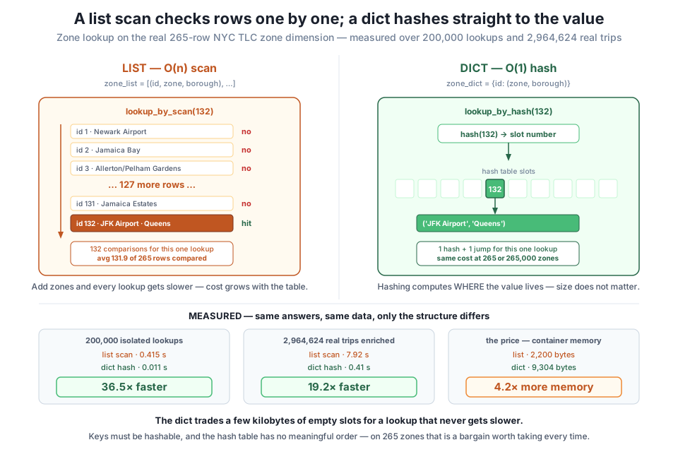
lookup_by_scan(132) started at row 1 and asked “is this it?” — Newark Airport, no. Jamaica Bay, no. Allerton/Pelham Gardens, no. It kept asking, 132 times, until it hit JFK Airport. It had no idea where id 132 lived, so it checked candidates one at a time until one matched. That is a linear scan, and its defining property is that the work is proportional to how much data there is. Formally, the cost is \( O(n) \) — double the zone table and you double the average lookup. Big-O notation is just this: a claim about how cost grows with size, ignoring constant factors.

lookup_by_hash(132) did something categorically different. It did not look at any zone row. It called hash(132), which chews the key through a fixed arithmetic routine and spits out a number, and then used that number to compute a slot — a position in a block of memory the dict keeps. It went to that slot and the value was sitting there. It never compared 132 against id 1, or id 2, or id 131, because it never had to consider them. It computed the address instead of searching for it.

That is what a hash table is, stripped of formalism: a structure where the key tells you where the value lives. You do not search, you calculate. And the consequence is the whole reason dicts matter — since hashing 132 costs the same whether the dict holds 265 entries or 265,000, the lookup cost does not grow with the size of the dict. That is \( O(1) \), constant time: not “fast” as a vague compliment, but “the same cost regardless of n” as a structural property.

(Two honest footnotes. Different keys can hash to the same slot — a collision — and the dict then does a little extra probing to sort it out; Python’s implementation keeps this rare enough that \( O(1) \) holds in practice, which is why you’ll see it written as average-case \( O(1) \). And the slots have to be allocated whether or not they are used, which is precisely the memory bill we settle at the end of this lesson.)

Let’s confirm the scan really is doing the work we claim. Time 200,000 lookups against each structure:

random.seed(7)
probes = [random.randint(1, 263) for _ in range(200_000)]

start = time.perf_counter()
for p in probes:
    lookup_by_scan(p)
scan_secs = time.perf_counter() - start

start = time.perf_counter()
for p in probes:
    lookup_by_hash(p)
hash_secs = time.perf_counter() - start

print(f"list scan : {scan_secs:6.3f} s   ({scan_secs / len(probes) * 1e6:6.3f} us per lookup)")
print(f"dict hash : {hash_secs:6.3f} s   ({hash_secs / len(probes) * 1e6:6.3f} us per lookup)")
print(f"dict is {scan_secs / hash_secs:.1f}x faster over {len(probes):,} lookups")

list scan :  0.415 s   ( 2.075 us per lookup)
dict hash :  0.011 s   ( 0.057 us per lookup)
dict is 36.5x faster over 200,000 lookups

36.5x, from changing a container. Both loops are the same shape and both call a Python function, so this is a like-for-like comparison — the only difference is what happens inside. And the per-lookup numbers explain themselves: 2.075 µs for the scan, 0.057 µs for the hash. The scan is not slow because looping is slow; it is slow because it does roughly 132 units of work where the dict does one:

position = {r["LocationID"]: i + 1 for i, r in enumerate(zone_records)}
avg_depth = sum(position[p] for p in probes) / len(probes)
print(f"average rows compared per list scan: {avg_depth:.1f} of {len(zone_list)}")

average rows compared per list scan: 131.9 of 265

131.9 rows compared per lookup, on average — half the table, which is exactly what you expect when the thing you want is equally likely to be anywhere in it. The dict compared none. That ratio, ~132 to 1, is the physical reason behind the 36.5x, and it is not a constant you can optimise away: it is half of len(zone_list). If CityFlow ever adopted a finer geography — census tracts instead of zones, say 2,000 rows — the scan would get roughly eight times slower and the dict would not move at all.

The Real Bill: 2,964,624 Trips#

A micro-benchmark is a claim; the pipeline is the test. Load every pickup location in the real month and enrich all of them, both ways.

start = time.perf_counter()
pickup_ids = pd.read_parquet("yellow_tripdata_2024-01.parquet", columns=["PULocationID"])["PULocationID"].tolist()
print(f"loaded {len(pickup_ids):,} real trips in {time.perf_counter() - start:.2f} s")

def boroughs_via_hash(ids):
    counts = Counter()
    for lid in ids:
        zone, borough = lookup_by_hash(lid)
        counts[borough] += 1
    return counts

def boroughs_via_scan(ids):
    counts = Counter()
    for lid in ids:
        zone, borough = lookup_by_scan(lid)
        counts[borough] += 1
    return counts

start = time.perf_counter()
hash_counts = boroughs_via_hash(pickup_ids)
enrich_hash_secs = time.perf_counter() - start

start = time.perf_counter()
scan_counts = boroughs_via_scan(pickup_ids)
enrich_scan_secs = time.perf_counter() - start

print(f"dict enrichment : {enrich_hash_secs:6.2f} s")
print(f"list enrichment : {enrich_scan_secs:6.2f} s")
print(f"same answer     : {hash_counts == scan_counts}")
print(f"end-to-end speedup: {enrich_scan_secs / enrich_hash_secs:.1f}x")
print("pickups by borough:")
for borough, n in hash_counts.most_common():
    print(f"  {borough:15s} {n:9,}")

loaded 2,964,624 real trips in 0.06 s
dict enrichment :   0.41 s
list enrichment :   7.92 s
same answer     : True
end-to-end speedup: 19.2x
pickups by borough:
  Manhattan       2,646,948
  Queens            273,128
  Brooklyn           25,258
  Unknown            12,018
  Bronx               6,905
  EWR                   295
  Staten Island          72

The whole month enriched in 0.41 s with the dict and 7.92 s with the list — identical borough counts, a 19.2x difference. (Yellow cabs are a Manhattan business: 89% of January’s pickups, with Queens’ 273,128 mostly airport runs. Ten kilobytes of zone table turned three million integers into something a dashboard can show.)

But look closely, because there is an honest discrepancy here and it teaches more than the headline does. The isolated benchmark said 36.5x. The real pipeline says 19.2x. Same structures, same machine — where did half the win go?

It went into the work that both versions do. The enrichment loop does not only look things up; it also iterates three million times and increments a Counter. That cost is identical in both versions, so it dilutes the ratio. Measure it directly:

def boroughs_via_nothing(ids):
    counts = Counter()
    for lid in ids:
        counts["all"] += 1
    return counts

start = time.perf_counter()
boroughs_via_nothing(pickup_ids)
overhead_secs = time.perf_counter() - start
print(f"shared loop overhead (iterate + count, no lookup): {overhead_secs:.2f} s")
hash_only = enrich_hash_secs - overhead_secs
scan_only = enrich_scan_secs - overhead_secs
print(f"lookup component, dict : {hash_only:6.2f} s")
print(f"lookup component, list : {scan_only:6.2f} s")
print(f"lookup-only ratio      : {scan_only / hash_only:.0f}x")

shared loop overhead (iterate + count, no lookup): 0.27 s
lookup component, dict : 0.15 s
lookup component, list : 7.65 s
lookup-only ratio      : 53x

There it is. Of the dict version’s 0.41 s, 0.27 s is not lookup at all — it is the price of visiting three million rows and counting them, which no data structure can refund. Strip that shared floor out and the lookup component alone is 0.15 s versus 7.65 s: a 53x ratio, back in line with the micro-benchmark.

All three numbers are true, and the discipline is knowing which one to quote. 53x is what the data structure did. 19.2x is what your pipeline felt. 36.5x was a benchmark measuring one operation with nothing else in the loop. Optimise a component that is 40% of your runtime and you cannot possibly win more than 40% back, no matter how good the optimisation — which is the same ceiling Module 5 hit when six processes delivered 3.96x instead of 6x. Speedups are always capped by the part you did not fix.

Sets: “Have I Seen This Trip Before?”#

Lookup has a sibling question that shows up in every ingest CityFlow runs: have I seen this record already? Feeds get replayed, a retried upload lands twice, a vendor resubmits a batch — and a dashboard that double-counts trips is worse than one that is late. So before loading, you dedup.

A set is the structure for this. It is a dict that kept the keys and threw away the values: same hash table, same constant-time membership test, no payload. k in some_set hashes k, jumps to the slot, and answers — without comparing k against anything else it holds.

Trips have no id column, so the key has to be composite — a tuple of the fields that together identify a trip. Vendor, pickup time, dropoff time, and the two location ids will do it: no two genuinely distinct trips plausibly share all five. Tuples are hashable as long as their contents are, so a tuple makes a perfect set member.

KEY_COLS = ["VendorID", "tpep_pickup_datetime", "tpep_dropoff_datetime", "PULocationID", "DOLocationID"]
trips = pd.read_parquet("yellow_tripdata_2024-01.parquet", columns=KEY_COLS + ["fare_amount", "total_amount"])
trip_keys = list(zip(
    trips["VendorID"].tolist(),
    trips["tpep_pickup_datetime"].astype("int64").tolist(),
    trips["tpep_dropoff_datetime"].astype("int64").tolist(),
    trips["PULocationID"].tolist(),
    trips["DOLocationID"].tolist(),
))
print("composite keys built:", f"{len(trip_keys):,}")
print("first key:", trip_keys[0])

def dedup_with_set(keys):
    seen = set()
    repeats = 0
    for k in keys:
        if k in seen:
            repeats += 1
        else:
            seen.add(k)
    return len(seen), repeats

start = time.perf_counter()
unique_n, repeat_n = dedup_with_set(trip_keys)
set_dedup_secs = time.perf_counter() - start
print(f"set dedup over {len(trip_keys):,} trips: {set_dedup_secs:.2f} s")
print(f"  distinct keys : {unique_n:,}")
print(f"  repeated keys : {repeat_n:,}  ({repeat_n / len(trip_keys) * 100:.2f}% of trips)")

composite keys built: 2,964,624
first key: (2, 1704070675000000, 1704071863000000, 186, 79)
set dedup over 2,964,624 trips: 0.52 s
  distinct keys : 2,933,515
  repeated keys : 31,109  (1.05% of trips)

Half a second to check three million trips against everything seen so far, and the answer is not zero: 31,109 repeated keys, 1.05% of the month. The timestamps became int64 nanoseconds via .astype("int64") — Timestamp objects are hashable and would have worked, but integers hash faster and the tuple gets smaller, which matters three million times over.

Why the List Version Is Not an Option#

Swap set for list and the code barely changes. seen = [], seen.append(k) instead of seen.add(k), and if k in seen reads identically. That last line is the trap: in is one word whether the container is a set or a list, and it hides two completely different algorithms. On a set it hashes and jumps. On a list it scans — and the list it scans is the pile of every trip seen so far, which is growing.

That changes the shape of the whole loop. Trip one scans nothing, trip 1,000 scans a thousand entries, trip 2,900,000 scans nearly three million. The total is the sum of that staircase, which is proportional to \( n^2 \) rather than \( n \) — this is \( O(n^2) \), and it is the difference between a job that finishes and a job that does not. Rather than assert it, watch it happen. Run both at 5,000, 10,000, 20,000, and 40,000 trips — doubling the input each time:

def dedup_with_list(keys):
    seen = []
    repeats = 0
    for k in keys:
        if k in seen:
            repeats += 1
        else:
            seen.append(k)
    return len(seen), repeats

print(f"{'n trips':>10} {'set (ms)':>10} {'list (ms)':>12} {'ratio':>9}")
list_secs_at = {}
for n in (5_000, 10_000, 20_000, 40_000):
    sub = trip_keys[:n]
    start = time.perf_counter()
    r_set = dedup_with_set(sub)
    t_set = time.perf_counter() - start
    start = time.perf_counter()
    r_list = dedup_with_list(sub)
    t_list = time.perf_counter() - start
    assert r_set == r_list
    list_secs_at[n] = t_list
    print(f"{n:10,} {t_set * 1000:10.2f} {t_list * 1000:12.1f} {t_list / t_set:8.0f}x")

   n trips   set (ms)    list (ms)     ratio
     5,000       0.42        170.7      409x
    10,000       0.74        661.7      899x
    20,000       1.75       2638.9     1505x
    40,000       3.22      10625.6     3302x

Read the two columns as sequences and the difference in kind jumps out. The set column doubles as the input doubles — 0.42, 0.74, 1.75, 3.22 — which is what \( O(n) \) total work looks like: each of the n membership tests costs the same, so n of them cost n. The list column quadruples: 170.7, 661.7, 2638.9, 10625.6. Double the trips and you pay four times, because you are doing twice as many scans and each scan is twice as long. That is \( O(n^2) \) in the wild.

And notice the ratio column is not a constant. It is 409x, then 899x, then 1505x, then 3302x — the penalty grows with your data. This is why “how slow is it?” is the wrong question for a list-based in. There is no answer; there is only an answer at a size. Project it out:

n_ref = 40_000
growth = len(trip_keys) / n_ref
projected = list_secs_at[n_ref] * growth ** 2
print()
print(f"list dedup at {n_ref:,} trips took {list_secs_at[n_ref]:.2f} s")
print(f"full month is {growth:.1f}x more trips, and the cost grows with the SQUARE:")
print(f"  projected list dedup on {len(trip_keys):,} trips: {projected:,.0f} s = {projected / 3600:.1f} hours")
print(f"  measured set  dedup on {len(trip_keys):,} trips: {set_dedup_secs:.2f} s")

list dedup at 40,000 trips took 10.63 s
full month is 74.1x more trips, and the cost grows with the SQUARE:
  projected list dedup on 2,964,624 trips: 58,368 s = 16.2 hours
  measured set  dedup on 2,964,624 trips: 0.52 s

The full month is 74.1x bigger than the 40,000-trip sample, so the list version costs \( 74.1^2 \) — about 5,500 times — more: roughly 16 hours, against the set’s measured 0.52 seconds. That projection is deliberately not measured, and you should treat its precision with suspicion: it is extrapolated from a single noisy 10.63 s timing, and rerunning this lesson has produced projections from 16 to 21 hours. But that spread is the least interesting thing about it. Sixteen hours or twenty-one, the conclusion is identical and it is not a tuning problem: one of these runs inside a nightly pipeline and the other cannot exist. Meanwhile all 10 cores from Module 5 would buy the list version a 10x at best — call it a two-hour dedup. Still hopeless. You cannot parallelize your way out of the wrong data structure. That is the whole argument of this module, in one comparison.

What the Duplicates Actually Are#

The set answered its question precisely: 31,109 keys occur more than once. It cannot answer the next question, which is whether a repeated key means a duplicate. That one is yours, and on real data it usually has a surprise in it. Group the fares by key — with a dict, naturally — and look:

fares = trips["fare_amount"].tolist()
groups = {}
for k, fare in zip(trip_keys, fares):
    groups.setdefault(k, []).append(fare)
repeated = {k: v for k, v in groups.items() if len(v) > 1}
print(f"keys appearing more than once : {len(repeated):,}")
print("group sizes:", Counter(len(v) for v in repeated.values()))
void_pairs = sum(1 for v in repeated.values() if sum(1 for f in v if f < 0) == 1)
looks_genuine = sum(1 for v in repeated.values() if all(f >= 0 for f in v))
print(f"  pairs where exactly one row has a negative fare (void + rebill): {void_pairs:,}")
print(f"  pairs where both rows are non-negative (genuine duplicates?)   : {looks_genuine:,}")

keys appearing more than once : 31,109
group sizes: Counter({2: 31109})
  pairs where exactly one row has a negative fare (void + rebill): 30,981
  pairs where both rows are non-negative (genuine duplicates?)   : 128

Every one of the 31,109 repeated keys occurs exactly twice — never three times — and in 30,981 of those pairs, one row carries a negative fare. Those are not duplicate trips at all. They are accounting reversals: a fare was charged, then voided with an equal and opposite row, exactly as a ledger does it. The key repeats because it is the same trip, but the second row is a correction, not a copy. Blindly calling set() on these and keeping the first of each pair would silently delete 30,981 voids and leave CityFlow’s revenue figures overstated — a data-quality bug born from a dedup that was technically correct and conceptually wrong.

Which leaves 128 pairs where both rows carry a non-negative fare. The obvious reading is that those are the real duplicates — the same trip recorded twice — and it is tempting to write that number down and move on. Don’t. That reading is an inference from one column, and the way to test an inference is to look at a second one. Open the suspects and print what they actually contain:

pairs = {}
for k, fare, total in zip(trip_keys, fares, trips["total_amount"].tolist()):
    pairs.setdefault(k, []).append((fare, total))
repeated_pairs = {k: v for k, v in pairs.items() if len(v) > 1}
suspects = [v for v in repeated_pairs.values() if all(f >= 0 for f, _ in v)]
print(f"the {len(suspects)} 'genuine duplicate' suspects, opened up (fare, total):")
for v in suspects[:5]:
    print("   ", v)
cancels = sum(1 for v in suspects if abs(v[0][1] + v[1][1]) < 0.01)
identical = sum(1 for v in repeated_pairs.values()
                if v[0][0] == v[1][0] and abs(v[0][1] - v[1][1]) < 0.01)
print(f"\n  suspects whose total_amount cancels to ~0 : {cancels} of {len(suspects)}")
print(f"  pairs identical in BOTH fare and total    : {identical}")

the 128 'genuine duplicate' suspects, opened up (fare, total):
    [(0.0, -4.0), (0.0, 4.0)]
    [(0.0, -4.0), (0.0, 4.0)]
    [(0.0, -1.5), (0.0, 1.5)]
    [(0.0, -1.0), (0.0, 1.0)]
    [(0.0, -1.5), (0.0, 1.5)]

  suspects whose total_amount cancels to ~0 : 120 of 128
  pairs identical in BOTH fare and total    : 0

They were never duplicates either. 120 of the 128 are reversals of zero-fare trips: the fare was 0.00 on both rows, so the sign test had nothing to catch, but the money moved in total_amount — a -4.00 cancelled by a +4.00, a toll or surcharge charged and voided. The remaining eight differ in fare or total, which makes them two distinct trips that happen to collide on all five key columns, not copies of one. And the count of pairs identical in both fare and total — an actual replayed record, the thing “duplicate” is supposed to mean — is zero.

So the honest answer for this month on this key is that there are no genuine duplicates at all. Every one of the 31,109 repeats is the ledger doing its job.

Sit with what just happened, because it is the more valuable half of this lesson. The set was right: 31,109 keys repeat, delivered in half a second over three million rows. The first interpretation was wrong — “31,109 duplicates” would have been a fabrication. But the second interpretation was wrong too: “30,981 voids and 128 real duplicates” is a more sophisticated number, it survives a sanity check, it sounds like the product of careful work, and it is still false. It failed for a mundane reason — it tested one column, and zero-fare rows are invisible to a test on fares. Only widening the evidence to total_amount exposed the last 120. The structure gives you the question cheaply; the interpretation is still engineering judgment — and judgment gets it wrong the first time, and sometimes the second. The discipline that saves you is not being clever. It is opening the rows and looking at them before you publish a number.

The Price: Memory, Hashability, Order#

Dicts and sets are not free, and an engineer who cannot state their cost is not really choosing them. Three prices, all real.

Memory. A hash table needs slots to hash into, and it deliberately keeps a good fraction of them empty — a full table would collide constantly and lose the \( O(1) \) that is its entire reason for existing. You are literally paying for emptiness. Measure it on both structures in this lesson:

print("zone dimension, 265 entries")
print(f"  list container : {sys.getsizeof(zone_list):8,} bytes")
print(f"  dict container : {sys.getsizeof(zone_dict):8,} bytes  ({sys.getsizeof(zone_dict) / sys.getsizeof(zone_list):.1f}x)")
seen_set = set(trip_keys)
seen_list = list(dict.fromkeys(trip_keys))
print(f"dedup structure, {len(seen_set):,} distinct trip keys")
print(f"  list container : {sys.getsizeof(seen_list) / 1e6:8.2f} MB")
print(f"  set container  : {sys.getsizeof(seen_set) / 1e6:8.2f} MB  ({sys.getsizeof(seen_set) / sys.getsizeof(seen_list):.2f}x)")

zone dimension, 265 entries
  list container :    2,200 bytes
  dict container :    9,304 bytes  (4.2x)
dedup structure, 2,933,515 distinct trip keys
  list container :    23.47 MB
  set container  :   134.22 MB  (5.72x)

The zone dict costs 4.2x the list’s container — and it is 9 kilobytes, so who cares: seven kilobytes bought a 19.2x on the pipeline. The dedup set is where it bites: 134.22 MB against 23.47 MB, a 5.72x overhead and 110 MB of real RAM to hold the same 2,933,515 keys. On this machine that is affordable. On a year of trips it would be 1.3 GB of pure bookkeeping, and Module 4’s memory discipline would start pushing back — which is exactly the tension Lesson 4 resolves into a decision guide. (These are sys.getsizeof container figures: the table itself, not the key tuples it points at, which both structures share. The container is what differs between the two, so it is what the comparison should isolate.)

Hashability. Keys must be hashable, which in practice means immutable. Tuples work; lists do not. {(2, 1704070675000000, 186): ...} is fine, {[2, 1704070675000000, 186]: ...} raises TypeError: unhashable type: 'list'. The reason is not arbitrary: a dict places a key by its hash, so a key that could change value after insertion would end up filed in a slot that no longer corresponds to it, and would become unfindable. Immutability is what makes the address stable. This is why our composite key is a tuple, and it is why NaN in a key is a genuine hazard — it is hashable but never equal to itself, so it can go in and never come out.

Order. The hash table’s slot order is a function of hash values, not of anything meaningful about your data. Python dicts do preserve insertion order (guaranteed since 3.7), which is a nice property of the implementation — but sets offer no such guarantee, and neither structure gives you sorted order or lets you ask for “the 10th entry.” If your access pattern is positional or ordered, a hash table is the wrong shape, and no amount of \( O(1) \) fixes that. The rest of this module is largely about what to reach for instead.

Practice Exercises#

Exercise 1 — Prove that \( O(1) \) really is independent of size. The lesson claims a dict lookup costs the same whether the dict holds 265 entries or far more. Test it. Build dicts of 265, 2,650, and 26,500 synthetic-id entries (pad the real zone data by offsetting LocationID — {lid + 1000 * k: value} — so the values stay real), and time 200,000 lookups against each. Then do the same with three equivalent lists and lookup_by_scan. Print both series and describe the shapes: one should be flat, the other should grow roughly 10x per step.

Exercise 2 — Find where the crossover is. A dict is not always worth it — building it costs a full pass. Write a function that takes a lookup count m, and compares (a) m scans against zone_list, versus (b) building zone_dict from zone_records and then doing m dict lookups. Time both for m in (1, 5, 25, 100, 500) and find the smallest m where the dict version wins overall. Explain in a comment why the crossover lands where it does.

Exercise 3 — Dedup on a different key and defend your choice. The lesson keyed on five columns, found 31,109 repeats, and discovered that none of them were duplicates — they were reversals. Try two other keys: a narrower one (VendorID, tpep_pickup_datetime, PULocationID) and a wider one (add fare_amount and total_amount to the five). Report the repeated-key count for each with a set, then inspect a few groups from the narrow key’s results. Which key would you actually dedup CityFlow’s ingest on, and what does each wrong choice cost — dropping real trips, or keeping duplicates?

Summary#

You replaced a scan with a jump and measured what it bought. A list lookup is \( O(n) \): it does not know where the answer is, so it compares candidates one by one — an average of 131.9 of the real zone table’s 265 rows per lookup. A dict is a hash table: hashing the key computes the slot the value lives in, so the lookup costs the same at 265 entries or 265,000 — \( O(1) \). Measured on the real NYC zone dimension, that is 0.415 s vs 0.011 s over 200,000 isolated lookups (36.5x), and 7.92 s vs 0.41 s enriching all 2,964,624 January 2024 trips (19.2x end to end — smaller because 0.27 s of loop-and-count overhead is shared by both; strip it out and the lookup component alone is 53x). Sets apply the same machinery to membership: deduping the month on a five-column composite key took 0.52 s and found 31,109 repeated keys, where a list-based in — whose cost grows as \( n^2 \), quadrupling from 170.7 ms to 10,625.6 ms as the input went 5,000 to 40,000 — projects to roughly 16 hours. Opening those repeats mattered twice over: a fare-sign test labelled 30,981 as void-plus-rebill pairs and 128 as genuine duplicates, but widening the evidence to total_amount showed 120 of those 128 were zero-fare reversals the sign test could not see and the last eight were distinct trips colliding on the key — leaving zero genuine duplicates. The structure found the question in half a second; the answer took two attempts. The price is measured too: 4.2x container memory for the zone dict, and 5.72x (134.22 MB vs 23.47 MB) for the dedup set, plus hashable keys and no meaningful ordering.

Key Concepts#

• Hash table — a structure where hashing the key computes where the value lives, so you calculate an address instead of searching for one. Dicts and sets are both hash tables; a set is a dict that kept the keys and dropped the values.
• \( O(1) \) vs \( O(n) \) — Big-O describes how cost grows with size. A dict lookup does not grow (constant); a list scan grows in proportion (linear). At 265 zones that is a 53x lookup difference; on a bigger dimension the gap widens on its own.
• The \( O(n^2) \) trap — if k in seen reads identically for a list and a set but hides two different algorithms. Against a growing list, each check scans everything seen so far, and total cost quadruples every time the input doubles: 0.52 s becomes a projected 16 hours on the same 2.96M trips.
• Composite keys must be hashable — tuples work as dict keys and set members, lists do not, because a mutable key could change after being filed and become unfindable. Convert timestamps to int64 for smaller, faster-hashing keys.
• The price of a hash table — deliberately empty slots keep collisions rare and \( O(1) \) honest, so you pay memory for speed: 4.2x on the 265-zone dict (9 KB — irrelevant), 5.72x on the 2.9M-key dedup set (110 MB — a real budget line).

Why This Matters#

Module 5 bought CityFlow 3.96x by using every core; this lesson bought 19.2x on the enrichment step by using the right container, on one core, with no new hardware. That ordering is the lesson: fix the algorithm before you scale the machine, because parallelism multiplies whatever work you hand it — including the work you did not need to do. The dedup makes the point unarguable. Ten cores would take the list-based version from ~16 hours to a still-impossible ~1.6; the set does it in 0.52 s on one. No amount of hardware rescues \( O(n^2) \), and recognising that shape before you write it is worth more than any tuning flag. The other half of the lesson is the dedup. The set delivered 31,109 repeated keys in half a second and it was right — but “repeated key” and “duplicate” are different claims, and every attempt to bridge them took another look at the data. The first reading, “31,109 duplicates,” was wrong. The second reading, “30,981 voids and 128 real duplicates,” was more careful, more plausible, and also wrong — it tested one column, and the zero-fare reversals were invisible to it. The true count of genuine duplicates is zero, and nothing but opening the rows would have revealed that. Fast structures make the questions cheap to ask; they never make the answers true. Choosing well means knowing both what the structure costs — the memory, the hashability, the lost order — and what it is actually telling you, which is usually less than you would like it to be.

Continue Building Your Skills#

The dict and the set both answer a question about identity: where does this key live, and have I seen it before. Neither has anything to say about order — and CityFlow’s pipeline is full of problems where order is the whole point. Lesson 2, Stacks & Queues, takes that on. You’ll meet LIFO and FIFO as access patterns rather than vocabulary, and then walk straight into a trap with the same character as the one you just escaped: list.pop(0) looks like the natural way to take the next item off a queue, and it is secretly \( O(n) \), because every remaining element has to shuffle down one position to fill the hole. Do it in a loop and you have rebuilt the quadratic disaster from this lesson wearing a different disguise. You’ll measure collections.deque against it and watch the same shape appear in the timings, then use a real queue to build the buffering and backpressure that let a streaming pipeline read faster than it can write without running out of memory. Same principle, new access pattern: match the structure to the question and the cost takes care of itself.