Title here
Summary here
CityFlow’s pipeline can now read a month of trips without drowning in memory (Module 4) and grind through them on every core at once (Module 5). But look closely at what those two modules never actually built: a place to put work. Module 4’s loop read a batch and immediately processed it. Module 5’s Pool was handed a finished list of six tasks before it started. Neither had to cope with the situation every real streaming pipeline lives in — batches arriving while earlier ones are still being processed, piling up somewhere, waiting their turn. That waiting area has a name. It’s a queue, and the order it hands work back out is not a detail; it is the whole design.
Two orders matter. FIFO (first in, first out) is what you want when work must be handled fairly in arrival order — the batch that showed up first gets processed first, and nothing starves while newer arrivals jump ahead. LIFO (last in, first out) is what you want when you need to unwind — undoing pipeline steps in reverse, or walking a structure without recursion. Python gives you both, but it also gives you a trap that is easy to fall into and painful to find: the obvious way to write a FIFO queue with a plain list is quadratic, and it looks perfectly fine until your queue gets big. This lesson proves that with real timings — a 200,000-element queue that takes 3,012.6 ms one way and 3.6 ms the other — then builds a real bounded buffer over all 2,964,624 January trips and explains what happens when the producer outruns the consumer.
By the end of this lesson, you will be able to:
list as a stack (LIFO) with append and pop, and explain why both are O(1) at the endlist.pop(0) is O(n) and measure the quadratic blow-up it causes when draining a queuecollections.deque for O(1) FIFO at both ends, and as a fixed-size sliding windowYou’ll need pyarrow, pandas, and Python’s standard library. Let’s give the pipeline somewhere to put things.
Everything below runs against CityFlow’s real month: January 2024 yellow-taxi trips from the NYC TLC Trip Record Data page, a public-domain dataset. Fetch it once and keep it next to your script — every runnable block reads the local copy by name:
# gate: skip
# CityFlow's month of yellow-taxi trips, fetched once from the public TLC site.
import urllib.request
urllib.request.urlretrieve(
    "https://d37ci6vzurychx.cloudfront.net/trip-data/yellow_tripdata_2024-01.parquet",
    "yellow_tripdata_2024-01.parquet",
)
Now open it and look at its shape — the row groups matter later, when we stream batches out of it:
import warnings
warnings.filterwarnings("ignore")

import gc
import resource
import time
import timeit
from collections import deque

import pandas as pd
import pyarrow.parquet as pq

MONTH = "yellow_tripdata_2024-01.parquet"
COLUMNS = ["tpep_pickup_datetime", "tpep_dropoff_datetime",
           "trip_distance", "fare_amount", "PULocationID"]

trip_file = pq.ParquetFile(MONTH)
print("file:      ", MONTH)
print("trips:     ", f"{trip_file.metadata.num_rows:,}")
print("row groups:", trip_file.metadata.num_row_groups)
print("rows each: ", [trip_file.metadata.row_group(i).num_rows
                      for i in range(trip_file.metadata.num_row_groups)])
file: yellow_tripdata_2024-01.parquet
trips: 2,964,624
row groups: 3
rows each: [1048576, 1048576, 867472]Just under three million trips in three row groups. That’s the stream CityFlow has to keep up with.
A stack is the simpler of the two structures, and Python’s list already is one. You add to the end with append and take from the end with pop(), and the last thing you pushed is the first thing you get back. That’s LIFO.
The reason a list is a good stack is where the work happens. A Python list is a contiguous block of pointers with spare capacity at the end. append writes into the next free slot; pop() hands back the last item and decrements the length. Neither one touches any other element, so both are O(1) — constant time, no matter whether the stack holds ten items or ten million. (append occasionally has to grow the underlying block, but that cost is spread across many appends, so it stays O(1) amortized.)
Here’s the shape of it, using the names of the steps CityFlow’s pipeline applies to a batch:
step_stack = []
for step in ["load_batch", "add_duration", "add_mph", "flag_suspect"]:
    step_stack.append(step)
    print(f"push {step:<13} depth={len(step_stack)}  top={step_stack[-1]}")

print("\nunwinding (last in, first out):")
while step_stack:
    print("  pop", step_stack.pop())
push load_batch depth=1 top=load_batch
push add_duration depth=2 top=add_duration
push add_mph depth=3 top=add_mph
push flag_suspect depth=4 top=flag_suspect
unwinding (last in, first out):
pop flag_suspect
pop add_mph
pop add_duration
pop load_batchNote step_stack[-1] — peeking at the top without removing it, also O(1). And notice the unwind order is the exact reverse of the push order. That reversal is not a quirk to work around; it is precisely what makes a stack the right tool for the next problem.
Toy stacks of strings don’t earn their keep. Here’s the real version of the problem.
CityFlow’s cleaning pipeline applies a series of steps to each batch, and the steps depend on each other. add_mph needs the duration_min column that add_duration created; flag_suspect needs the mph column that add_mph created. Now suppose a step fails validation partway through and you need to return the batch to its original state — you cannot undo them in any order. You must undo flag_suspect before add_mph, and add_mph before add_duration, because each step’s undo assumes the later steps are already gone. Reverse order of application. That is LIFO, and a stack enforces it for free.
So each step, as it runs, pushes an undo record — its name and a function that reverses it — onto a stack. Load a real batch and apply all three:
batch = next(trip_file.iter_batches(batch_size=50_000, columns=COLUMNS)).to_pandas()
print("batch loaded:", batch.shape)

undo_stack = []

def add_duration(frame):
    frame["duration_min"] = (
        frame["tpep_dropoff_datetime"] - frame["tpep_pickup_datetime"]
    ).dt.total_seconds() / 60.0
    undo_stack.append(("add_duration", lambda f: f.drop(columns=["duration_min"])))
    return frame

def add_mph(frame):
    frame["mph"] = frame["trip_distance"] / (frame["duration_min"] / 60.0).replace(0, float("nan"))
    undo_stack.append(("add_mph", lambda f: f.drop(columns=["mph"])))
    return frame

def flag_suspect(frame):
    frame["suspect"] = (frame["mph"] > 80) | (frame["duration_min"] <= 0)
    undo_stack.append(("flag_suspect", lambda f: f.drop(columns=["suspect"])))
    return frame

for step_fn in (add_duration, add_mph, flag_suspect):
    batch = step_fn(batch)
    print(f"applied {undo_stack[-1][0]:<13} columns={len(batch.columns)}  undo depth={len(undo_stack)}")

print("\nsuspect trips flagged:", int(batch["suspect"].sum()), "of", f"{len(batch):,}")
batch loaded: (50000, 5)
applied add_duration columns=6 undo depth=1
applied add_mph columns=7 undo depth=2
applied flag_suspect columns=8 undo depth=3
suspect trips flagged: 36 of 50,000Five columns became eight, and the pipeline flagged 36 physically implausible trips out of 50,000 — trips recorded at over 80 mph or with a non-positive duration. The undo stack is three deep. Now unwind it:
print("rolling back:")
while undo_stack:
    name, undo_fn = undo_stack.pop()
    batch = undo_fn(batch)
    print(f"  undid {name:<13} columns now {len(batch.columns)}")

print("\nback to the original batch:", list(batch.columns))
rolling back:
undid flag_suspect columns now 7
undid add_mph columns now 6
undid add_duration columns now 5
back to the original batch: ['tpep_pickup_datetime', 'tpep_dropoff_datetime', 'trip_distance', 'fare_amount', 'PULocationID']Eight columns back to the original five, in strictly reverse order, and the rollback loop never had to know the order — the stack remembered it. This is the same mechanism behind a database transaction’s rollback log, an editor’s undo button, and the call stack your Python program runs on right now. It’s also how you traverse a tree without recursion: push the children, pop one, push its children, repeat until the stack empties. Module 7 leans on exactly that when recursion gets too deep.
Now the other order. A queue hands work back in arrival order — first in, first out — which is what CityFlow’s streaming pipeline needs. A batch that arrived at 09:00 should be processed before one that arrived at 09:05, or the dashboard shows stale numbers for the oldest data while the newest sails through.
The obvious way to write that with a list is to append to the end and pop(0) from the front. It works, and it reads beautifully:
work_queue = ["batch_01", "batch_02", "batch_03", "batch_04"]
print("arrived:", work_queue)
while work_queue:
    job = work_queue.pop(0)
    print(f"  processing {job}   still waiting: {len(work_queue)}")
arrived: ['batch_01', 'batch_02', 'batch_03', 'batch_04']
processing batch_01 still waiting: 3
processing batch_02 still waiting: 2
processing batch_03 still waiting: 1
processing batch_04 still waiting: 0Correct FIFO. Four batches in, four batches out, oldest first. If your queue never exceeds a handful of items, this code is genuinely fine and you should not lose sleep over it.
But pop(0) hides a cost that pop() doesn’t have, and it comes straight from how a list is built. A list is a contiguous array of pointers, and its defining property is that element i lives at a fixed offset from the start — that’s what makes work_queue[i] an O(1) lookup. Removing the last element preserves that property for free. Removing the first element does not: element 1 must become element 0, element 2 must become element 1, and so on. Every remaining element shifts one slot left. That is O(n) work for a single pop(0).
Now drain a whole queue of items. The first pop shifts elements, the second shifts , and so on:
Draining the queue is quadratic. Double the queue and the work quadruples. collections.deque — a double-ended queue — is built differently: it’s a doubly-linked list of small blocks, so removing from the front just unlinks a block and moves a pointer. Nothing shifts. popleft() is O(1), and draining is linear.
That’s the theory. Let’s find out whether it’s true.
Same job both ways — fill a queue with integers, then pop every one of them off the front until it’s empty — timed at four sizes:
def drain_with_list(n):
    queue = list(range(n))
    start = time.perf_counter()
    while queue:
        queue.pop(0)
    return time.perf_counter() - start

def drain_with_deque(n):
    queue = deque(range(n))
    start = time.perf_counter()
    while queue:
        queue.popleft()
    return time.perf_counter() - start

print(f"{'queue size':>11} {'list.pop(0)':>13} {'deque.popleft()':>16} {'deque faster by':>16}")
timings = []
for n in (10_000, 50_000, 100_000, 200_000):
    list_secs = drain_with_list(n)
    deque_secs = drain_with_deque(n)
    timings.append((n, list_secs, deque_secs))
    print(f"{n:>11,} {list_secs*1000:>11.1f}ms {deque_secs*1000:>14.1f}ms {list_secs/deque_secs:>15.0f}x")
queue size list.pop(0) deque.popleft() deque faster by
10,000 5.2ms 0.2ms 30x
50,000 182.1ms 0.9ms 201x
100,000 780.0ms 2.2ms 351x
200,000 3012.6ms 3.6ms 829xRead the two columns downward and you can see the difference in kind, not just degree. Twenty times more elements (10,000 to 200,000) cost the list 580 times more work — 5.2 ms to 3,012.6 ms. The same twenty-fold increase cost the deque about 18 times more — 0.2 ms to 3.6 ms, near enough to linear. The gap between them widens from 30x to 829x as the queue grows, and it keeps widening; there is no size at which the list catches up.
The cleanest way to see an algorithmic complexity is to double the input and watch what happens to the time. Linear work doubles. Quadratic work quadruples:
print("when the queue DOUBLES, how much does the drain time grow?")
print(f"{'size step':>20} {'list':>10} {'deque':>10}")
for i in range(1, len(timings)):
    n_prev, l_prev, d_prev = timings[i - 1]
    n_now, l_now, d_now = timings[i]
    print(f"{n_prev:>8,} -> {n_now:<8,} {l_now/l_prev:>8.2f}x {d_now/d_prev:>9.2f}x")
when the queue DOUBLES, how much does the drain time grow?
size step list deque
10,000 -> 50,000 34.88x 5.20x
50,000 -> 100,000 4.28x 2.45x
100,000 -> 200,000 3.86x 1.64xThere is the proof, and it is about as textbook as real measurements ever get. Look at the two genuine doublings: 50,000 to 100,000 costs the list 4.28x more time, and 100,000 to 200,000 costs 3.86x more. Both hover around 4 — and is exactly the signature of . The deque’s same doublings cost 2.45x and 1.64x, hovering around 2: linear. The first row is a five-fold size jump rather than a doubling, so its expected ratios are for quadratic and 5 for linear; the measured 34.88x and 5.20x bracket those well.
Be honest about the noise, though. The deque’s numbers are sub-millisecond, so timer granularity and background load move them around by a few percent — 2.45x and 1.64x average out near 2, but individually they wobble. The list’s numbers are large enough that the quadratic signal swamps any noise. The ratios are the point, and the ratios hold.
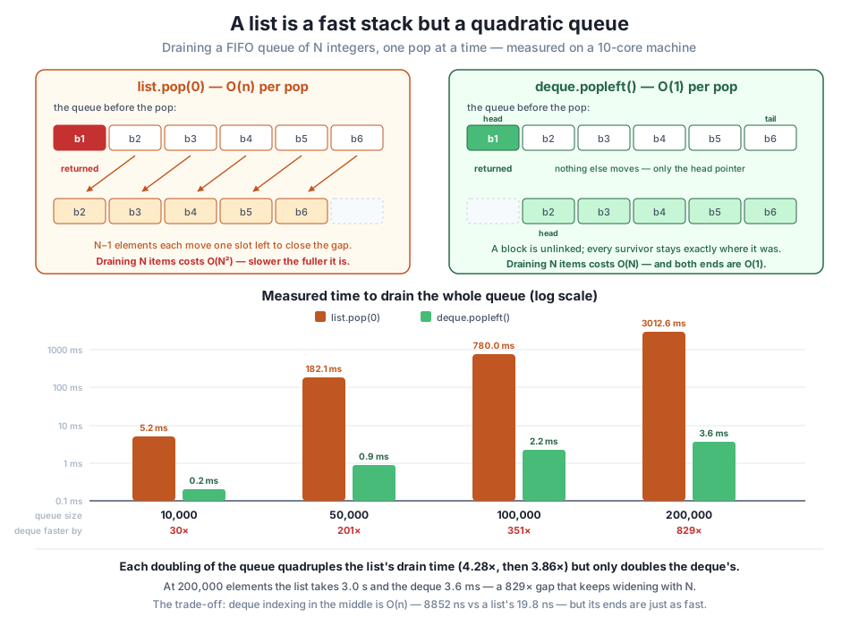
list.pop(0) returns the front element and then shifts every one of the N−1 survivors one slot left to close the gap — O(n) per pop, so O(N²) to drain. Right: deque.popleft() unlinks a block and moves the head pointer; nothing else moves — O(1) per pop, O(N) to drain. The chart shows the consequence: each doubling of the queue quadruples the list's drain time (4.28×, then 3.86× — the signature of quadratic growth) but only doubles the deque's. At 200,000 elements the list takes 3,012.6 ms and the deque 3.6 ms, a 829× gap that keeps widening with N. The trade-off is real but narrow: indexing a deque in the middle is O(n) (8,852 ns vs a list's 19.8 ns), while its ends are just as fast. Exact times vary by machine and run; the ratios are the point.The trap is that it looks fine in testing
This is the single most common accidental-quadratic bug in Python data code, and its danger is entirely about scale. At 10,000 elements list.pop(0) drains in 5.2 ms — you will never notice it, and no test will fail. At 200,000 it takes 3 s. At two million it would take roughly a hundred times that, because the cost grows with the square. A pipeline that was instant on a test fixture quietly becomes a production incident on a real backlog, and the profiler points at a line of code that looks completely innocent. The rule is simple enough to adopt permanently: if you pop from the front, use a deque. The import is free and the code is otherwise identical.
Now put the deque to work where CityFlow actually needs it. A streaming pipeline has a producer (something reading batches out of the parquet file) and a consumer (something processing them). The buffer between them is the queue, and its size is a design decision with real consequences.
deque takes a maxlen argument that makes it bounded: once it holds maxlen items, appending one pushes the oldest out the other end. Here the producer appends each batch and the consumer pops the oldest as soon as the buffer is full, streaming all three row groups through a buffer that never holds more than two batches:
def peak_rss_mb():
    return resource.getrusage(resource.RUSAGE_SELF).ru_maxrss / (1024 * 1024)

del batch
gc.collect()
baseline_mb = peak_rss_mb()
print("peak RSS before any buffering:", f"{baseline_mb:.0f} MB")

bounded_buffer = deque(maxlen=2)
batches_seen = 0
trips_processed = 0
fare_total = 0.0

for arrow_batch in pq.ParquetFile(MONTH).iter_batches(batch_size=50_000, columns=COLUMNS):
    bounded_buffer.append(arrow_batch.to_pandas())          # producer
    batches_seen += 1
    if len(bounded_buffer) == bounded_buffer.maxlen:
        ready = bounded_buffer.popleft()                    # consumer
        trips_processed += len(ready)
        fare_total += float(ready["fare_amount"].sum())

while bounded_buffer:                                       # drain the tail
    ready = bounded_buffer.popleft()
    trips_processed += len(ready)
    fare_total += float(ready["fare_amount"].sum())

bounded_peak = peak_rss_mb()
print("\nbounded buffer - deque(maxlen=2):")
print("  batches streamed: ", batches_seen)
print("  trips processed:  ", f"{trips_processed:,}")
print("  total fares:      ", f"${fare_total:,.2f}")
print("  peak RSS:         ", f"{bounded_peak:.0f} MB",
      f"(+{bounded_peak - baseline_mb:.0f} MB over baseline)")
gc.collect()
peak RSS before any buffering: 129 MB
bounded buffer - deque(maxlen=2):
batches streamed: 60
trips processed: 2,964,624
total fares: $53,882,224.76
peak RSS: 168 MB (+39 MB over baseline)All 2,964,624 trips — every single one, none dropped — streamed through a buffer holding at most two batches, totalling $53,882,224.76 in fares. The popleft() is FIFO: the batch that has waited longest is always the one processed next.
Now the counterfactual. Change one thing — use a plain list and never pop — and you have the version an unwary engineer writes when they want to “collect the batches first and process them after”:
unbounded_buffer = []
for arrow_batch in pq.ParquetFile(MONTH).iter_batches(batch_size=50_000, columns=COLUMNS):
    unbounded_buffer.append(arrow_batch.to_pandas())

held_mb = sum(f.memory_usage(deep=True).sum() for f in unbounded_buffer) / 1e6
unbounded_peak = peak_rss_mb()
print("unbounded buffer - a plain list:")
print("  batches held:", len(unbounded_buffer))
print("  data held:   ", f"{held_mb:.0f} MB")
print("  peak RSS:    ", f"{unbounded_peak:.0f} MB",
      f"(+{unbounded_peak - baseline_mb:.0f} MB over baseline)")
print(f"\nbuffer's own cost: {held_mb:.0f} MB held vs ~{2 * 1.8:.1f} MB for the bounded deque")
print(f"peak RSS difference: {unbounded_peak - bounded_peak:.0f} MB")
del unbounded_buffer
gc.collect()
unbounded buffer - a plain list:
batches held: 60
data held: 107 MB
peak RSS: 277 MB (+147 MB over baseline)
buffer's own cost: 107 MB held vs ~3.6 MB for the bounded deque
peak RSS difference: 109 MBSame 60 batches, same trips, same answer — and 107 MB of resident memory held for no reason. The peak RSS difference between the two runs is 109 MB, which matches the 107 MB the buffer accumulated almost exactly. The bounded version holds two batches: about 3.6 MB.
One honest caveat about those RSS numbers, because it’s a lesson in itself. The bounded run still shows +39 MB over its baseline, and none of that is the deque — it’s pyarrow decoding a full row group (1,048,576 rows) to serve you 50,000-row batches, plus allocator overhead. ru_maxrss is a high-water mark that never goes down, which is exactly why the bounded run is measured first here: the difference between the two peaks is attributable to the buffer, but the absolute numbers include everything the process ever touched. When you attribute memory, attribute it to the thing that actually grew.
And 107 MB is the small version of this problem. That’s one month. CityFlow’s dashboard covers years, and the unbounded buffer’s memory grows with the length of the stream — which is another way of saying it grows without bound. This is Module 1’s memory wall arriving through the back door: not from loading one file too big for RAM, but from a queue that quietly keeps everything it was ever handed. An unbounded queue in a long-running pipeline is a memory leak waiting to happen, and it fails at the worst possible moment — after hours of successful processing, when the stream finally gets long enough.
The bounded buffer raises the obvious question. If the producer is faster than the consumer — batches arrive quicker than they get processed — the buffer fills. What then?
That question has a name: backpressure. It’s the signal that travels backwards from a full consumer to an eager producer, telling it to slow down. Every streaming system has to answer it, and there are only three possible answers: drop the new work, drop the old work, or make the producer wait.
deque(maxlen=...) picks one of those answers for you, silently, and you need to know which:
overflow = deque(maxlen=3)
for name in ["batch_01", "batch_02", "batch_03", "batch_04", "batch_05"]:
    dropped = overflow[0] if len(overflow) == overflow.maxlen else None
    overflow.append(name)
    note = f"  <- pushed {dropped} out" if dropped else ""
    print(f"append {name}  buffer={list(overflow)}{note}")

print("\nbatch_01 and batch_02 were silently discarded - never processed, no error raised.")
append batch_01 buffer=['batch_01']
append batch_02 buffer=['batch_01', 'batch_02']
append batch_03 buffer=['batch_01', 'batch_02', 'batch_03']
append batch_04 buffer=['batch_02', 'batch_03', 'batch_04'] <- pushed batch_01 out
append batch_05 buffer=['batch_03', 'batch_04', 'batch_05'] <- pushed batch_02 out
batch_01 and batch_02 were silently discarded - never processed, no error raised.maxlen drops the oldest item, with no exception and no warning. For a sliding window over recent data — the last 5 fares, the last 100 GPS pings — that is exactly the behaviour you want; old data ageing out is the definition of the window. For a work queue it is data loss, and the fact that it is silent makes it worse than a crash. In the streaming buffer above this was safe only because the consumer popped on every iteration, so the buffer never actually overflowed.
When you need real backpressure — the producer waits instead of losing data — reach for queue.Queue(maxsize=N) from the standard library, whose put() blocks when the queue is full until a consumer makes room. That blocking is the backpressure: the producer physically cannot run ahead. queue.Queue is also thread-safe, which matters once the producer and consumer are the separate threads Module 5 introduced. The design question to answer before you pick is always the same: when the consumer falls behind, what is allowed to happen? Bounded-and-blocking (slow down), bounded-and-dropping (lose data, bound memory), or unbounded (keep everything, and eventually die). There is no fourth option, and refusing to choose means choosing the third by default.
The left in popleft is the tell. A deque isn’t just a queue — it’s a double-ended queue, O(1) at both ends. append/pop work the right end; appendleft/popleft work the left. That’s what lets one structure be a stack, a queue, and a sliding window.
The sliding window is the elegant one. Combine maxlen with append and the “drop the oldest” behaviour that was dangerous for a work queue becomes exactly right — a fixed-size window over a stream that maintains itself, with no bookkeeping at all:
window = deque(maxlen=5)
sample = next(pq.ParquetFile(MONTH).iter_batches(batch_size=20, columns=COLUMNS)).to_pandas()
print(f"{'fare':>8} {'window':>8} {'rolling mean':>14}")
for fare in sample["fare_amount"].head(10):
    window.append(float(fare))
    print(f"{fare:>8.2f} {len(window):>8} {sum(window)/len(window):>13.2f}")
fare window rolling mean
17.70 1 17.70
10.00 2 13.85
23.30 3 17.00
10.00 4 15.25
7.90 5 13.78
29.60 5 16.16
45.70 5 23.30
25.40 5 23.72
31.00 5 27.92
3.00 5 26.94A 5-trip rolling mean of real fares, and the window manages itself — it grows to 5 and then stays there forever, each new fare evicting the oldest. No index arithmetic, no slicing, no manual truncation. That’s a genuine streaming rolling statistic: it works on an infinite stream in constant memory, which pandas.rolling cannot do because it needs the whole column in memory first.
So why not use a deque everywhere? Because every structure trades something, and the deque’s trade is precise. Those linked blocks that make the ends O(1) mean there’s no single contiguous array to compute an offset into. To reach the middle, a deque has to walk — block by block. Indexing a deque in the middle is O(n):
size = 200_000
as_list = list(range(size))
as_deque = deque(range(size))
middle = size // 2
reps = 200_000

list_mid = timeit.timeit(lambda: as_list[middle], number=reps) / reps * 1e9
deque_mid = timeit.timeit(lambda: as_deque[middle], number=reps) / reps * 1e9
deque_end = timeit.timeit(lambda: as_deque[0], number=reps) / reps * 1e9

print(f"list[{middle:,}]   {list_mid:>9.1f} ns   O(1) - one offset from the start")
print(f"deque[{middle:,}]  {deque_mid:>9.1f} ns   O(n) - walks block by block")
print(f"deque[0]         {deque_end:>9.1f} ns   O(1) - it is an end")
print(f"\nin the middle, deque is {deque_mid / list_mid:.0f}x slower than list")
print(f"at the ends, they are within {abs(deque_end - list_mid):.0f} ns of each other")
list[100,000] 19.8 ns O(1) - one offset from the start
deque[100,000] 8852.3 ns O(n) - walks block by block
deque[0] 22.8 ns O(1) - it is an end
in the middle, deque is 447x slower than list
at the ends, they are within 3 ns of each otherThe symmetry with the queue result is almost poetic. The list beat the deque by 447x at random access in the middle; the deque beat the list by 829x at FIFO draining. Neither structure is “faster” — each is faster at the access pattern it was built for, and catastrophically slower at the other one. And notice deque[0] costs 22.8 ns against the list’s 19.8 ns: at the ends they’re within 3 ns, which is noise. The deque’s penalty is not “indexing is slow,” it’s specifically “indexing away from the ends is slow.”
That’s the whole decision rule. If you scan and pop from the ends, use a deque. If you need random access by position, use a list. If you find yourself wanting both on the same large structure, that’s a signal you may want a different structure entirely — which is exactly the question Lesson 4 takes up.
Exercise 1 — Find the size where the trap starts to bite. The lesson measured list.pop(0) at 10,000 through 200,000. Extend drain_with_list and drain_with_deque down to smaller sizes — try 100, 500, 1,000, and 5,000 — and print the ratio at each. Find roughly where the list stops being competitive. Then explain in a comment why list.pop(0) is a perfectly defensible choice for a queue of 50 items, and what property of means the answer is a threshold rather than “never use a list.”
Hint
Reuse both functions unchanged and loop over (100, 500, 1_000, 5_000, 10_000). At the smallest sizes the timings will be microseconds and the ratio may even favour the list, because a deque node carries more per-element overhead and the list’s shift is a single fast memmove of a tiny block. Quadratic growth is about the rate, not any single point: is small when is small. The threshold is where the curve’s steepness overtakes the constant factor — which is why “measure at your real size” beats memorising a rule.
Exercise 2 — Make the buffer actually overflow, and count the loss. Rewrite the streaming buffer so the consumer is slower than the producer: use deque(maxlen=4), append every batch, but only pop and process on every third iteration. Track how many trips you processed versus the 2,964,624 that were produced, and report how many were silently dropped by maxlen. Then change the structure to queue.Queue(maxsize=4) and explain in a comment what would happen differently on the put() call.
Hint
Compare trips_processed against trip_file.metadata.num_rows — the gap is your data loss, and maxlen will not tell you about it. To detect the drop as it happens, check len(bounded_buffer) == bounded_buffer.maxlen before appending, as the overflow demo does. With queue.Queue(maxsize=4), put() would block forever waiting for room that a single-threaded loop can never make — which is precisely the point: blocking is backpressure, and a deadlock here is the structure telling you the producer and consumer need to be separate threads.
Exercise 3 — Build a streaming anomaly detector with a sliding window. Use deque(maxlen=100) to hold the last 100 trip_distance values as you stream one row group with iter_batches. For each new trip, before appending it, compare it to the current window’s mean; flag it if it is more than 5 times that mean. Report how many trips you flagged, and explain in a comment why a deque makes this possible on a stream of any length while a pandas.rolling call would not.
Hint
Guard the early iterations — the window is empty at first, so require len(window) == window.maxlen before you judge anything. Compute the mean with sum(window) / len(window); it’s 100 floats, so the cost is trivial. The key insight for your comment: the deque holds a constant 100 values no matter how many million trips flow past, so memory is O(1) in the stream length, while pandas.rolling needs the entire column resident before it computes anything — the Module 1 memory wall again. (If you want the window’s mean in O(1) too, keep a running sum: add the new value, subtract the one maxlen evicts.)
You gave CityFlow’s pipeline somewhere to put work, and learned that the container’s order is a design decision. A stack is LIFO — list.append and list.pop(), both O(1) because they touch only the end — and it’s the right tool whenever you must unwind: you rolled back three interdependent pipeline steps on a real 50,000-trip batch (which flagged 36 implausible trips) in exactly reverse order, without the rollback loop needing to know that order. A queue is FIFO, and it hides the trap: list.pop(0) is O(n) because every remaining element shifts left to close the gap, making a full drain . The measurements were unambiguous — 5.2 ms at 10,000 elements but 3,012.6 ms at 200,000, quadrupling (4.28x, then 3.86x) on each doubling, while deque.popleft() stayed linear at 3.6 ms for a 829x gap that widens with every added element. You then streamed all 2,964,624 January trips ($53,882,224.76 in fares) through a deque(maxlen=2), and saw the unbounded version hold 107 MB it never needed — Module 1’s memory wall arriving through a queue that keeps everything. Finally, the honest trade: deque is O(1) at both ends, which makes it a queue and a sliding window at once, but indexing its middle costs 8,852 ns against a list’s 19.8 ns — 447x slower — while its ends match the list to within 3 ns.
append and pop() at the end, both O(1). The right structure whenever order must be reversed: undo logs, transaction rollback, iterative traversal, and the call stack itself.pop(0) trap — a list is a contiguous array, so removing the front shifts all N−1 survivors: O(n) per pop, to drain. Fine at 50 items, a 3-second stall at 200,000, and it looks innocent in code review.collections.deque — a linked list of blocks: append/appendleft/pop/popleft are all O(1), so it is a stack, a FIFO queue, and a sliding window in one. Indexing its middle is O(n) — the price of having two cheap ends.deque(maxlen=N) silently drops the oldest, queue.Queue(maxsize=N) blocks the producer, and an unbounded queue grows with the stream until the process dies.The queue trap is worth internalising because of how it fails rather than how badly. A pipeline using list.pop(0) passes every test, sails through code review, and runs beautifully for months — until the day a backlog builds and a queue that used to hold 200 items holds 200,000, and a job that took a second takes an hour. Nothing changed but the data, and the profiler blames a line that is obviously correct. That is the characteristic shape of a complexity bug, and the defence is the habit this module keeps drilling: know the access pattern your code performs, and know what that pattern costs in the structure you chose. The deeper point is that there is no “best” structure, only a best fit — the same list that lost by 829x as a queue won by 447x at random access. Choosing well is not about memorising which one is fast; it’s about naming your access pattern honestly, then picking the structure whose cheap operations are the ones you actually perform. The bounded-buffer question sharpens the same judgment: “what happens when the consumer falls behind?” has three answers, and a pipeline that never asks has silently chosen the one that runs out of memory.
Your queue now hands work back in arrival order, fairly and in O(1) — but fair is not always what CityFlow needs. When the dashboard asks for the ten busiest pickup zones out of 265, or when a backlog of batches has to be worked in order of urgency rather than arrival, FIFO is the wrong discipline entirely; you need whatever is most important next, no matter when it arrived. Lesson 3, Heaps & Priority Queues, introduces the structure that delivers exactly that: heapq, which keeps the smallest (or largest) item always one O(1) peek away and costs only to insert. You’ll use it to answer top-N questions without sorting everything you own — the reason a bounded heap can find the busiest zones in a stream of millions while holding only N items in memory, and why that beats a full sort by a margin you’ll measure for yourself. It is the same trade you just made with the deque, applied to a new access pattern: give up the operations you don’t need, and the one you do gets dramatically cheaper.
Keep DATATWEETS free. Help fund practical data, AI, and engineering lessons for learners worldwide.
