Title here
Summary here
CityFlow’s dashboard opens with a single panel: the 10 busiest pickup zones this month. You already have everything you need to build it. Lesson 1 gave you a dict that maps a LocationID to a zone name in O(1), and Module 4 taught you to stream a month of trips through iter_batches without ever holding it in memory. Counting trips per zone is a Counter and one pass. Then comes the last step, and almost everyone writes the same line: sort the counts and take the first ten. It works. It is also the moment worth stopping on, because you just asked Python to put all 260 zones into perfect order — to decide whether the 187th busiest zone outranks the 188th — in order to answer a question that never asked about either of them. You did O(n log n) work to report ten rows.
There is a data structure whose entire purpose is that mismatch. A heap keeps one element — the smallest — instantly available and deliberately leaves everything else only roughly arranged, which is exactly the trade you want when you care about the extremes and not the middle. This lesson builds the intuition honestly: what a heap really is (a tree flattened into an ordinary list, and you’ll see a printout proving it is not sorted), how heapq exposes it, and then measurements that refuse to flatter the technique. On CityFlow’s 260 zones the heap saves about six microseconds, which is nothing, and this lesson says so plainly. Then it goes to where the structure actually earns its place: finding the ten biggest tips among 2,964,624 trips, where a full sort takes 1.205 s and a heap takes 0.066 s — and, more importantly, a bounded heap running over Module 4’s stream answers the same question in 10.6 MB instead of 313.1 MB, on data that never has to fit in memory at all.
By the end of this lesson, you will be able to:
heappush, heappop, heapify, and heappushpop, and explain why heapify is O(n) rather than O(n log n)(priority, item) tuples, avoid the tie-break TypeError, and get max-heap behaviour out of Python’s min-heapYou’ll need pyarrow, pandas, and Python’s standard library. Let’s stop sorting things nobody asked about.
Start where Module 4 left off: one streaming pass over the January month, counting pickups per zone, joined to human-readable names through Lesson 1’s dict. Nothing here is new — it is the input to the interesting part.
The trip month and the zone dimension come from the NYC TLC Trip Record Data page; the zone lookup is served from our own stable mirror. Fetch them once next to your script — every runnable block below reads the local copies by plain name:
# gate: skip
# CityFlow's January trips and the zone dimension, fetched once.
import urllib.request
urllib.request.urlretrieve(
    "https://d37ci6vzurychx.cloudfront.net/trip-data/yellow_tripdata_2024-01.parquet",
    "yellow_tripdata_2024-01.parquet")
urllib.request.urlretrieve(
    "https://datatweets.com/datasets/nyc-taxi/taxi_zone_lookup.csv",
    "taxi_zone_lookup.csv")
Now the counting pass:
import warnings
warnings.filterwarnings("ignore")
import heapq
import time
from collections import Counter
from itertools import count
import pandas as pd
import pyarrow.parquet as pq

TRIPS = "yellow_tripdata_2024-01.parquet"
zones = pd.read_csv("taxi_zone_lookup.csv")
zone_name = dict(zip(zones["LocationID"], zones["Zone"]))

start = time.perf_counter()
counts = Counter()
for batch in pq.ParquetFile(TRIPS).iter_batches(batch_size=250_000, columns=["PULocationID"]):
    counts.update(batch.column("PULocationID").to_pylist())
count_secs = time.perf_counter() - start

pairs = [(n, zone_name.get(z, "Unknown")) for z, n in counts.items()]
print(f"trips counted         : {sum(counts.values()):,}")
print(f"distinct pickup zones : {len(pairs)}")
print(f"one streaming pass    : {count_secs:.2f}s")
print(f"first 3 pairs (arrival order): {pairs[:3]}")
trips counted : 2,964,624
distinct pickup zones : 260
one streaming pass : 0.64s
first 3 pairs (arrival order): [(104523, 'Penn Station/Madison Sq West'), (66060, 'Lenox Hill East'), (136465, 'Upper East Side North')]Just under three million trips reduced to 260 (count, zone) pairs in 0.64 s, and note the shape of that data: (count, zone) with the count first. That ordering is deliberate and it matters for everything that follows — Python compares tuples element by element, so ordering these pairs means ordering them by trip count, with the zone name as an automatic alphabetical tie-break. The pairs arrive in whatever order the zones first appeared in the data, which is to say no useful order at all. The dashboard needs the top ten of them.
A heap is a binary tree with one rule, called the heap invariant: every parent is less than or equal to both of its children. That is the whole definition. Notice what it does not say — it says nothing about the relationship between siblings, or between cousins, or between a node on the left of the tree and a node on the right. It constrains only the vertical relationship, parent to child. Follow that rule from any starting point and you can only walk downhill to bigger values, which means the single smallest element in the entire structure has nowhere to hide: it must sit at the root.
The second half of the idea is the part that makes heaps fast in practice: the tree is not a tree. There are no node objects and no pointers. The tree is flattened into an ordinary Python list by reading it top-to-bottom, left-to-right, so that the item at index \( i \) has its children at indices \( 2i+1 \) and \( 2i+2 \), and its parent at \( \lfloor (i-1)/2 \rfloor \). Position is structure. The root — the minimum — is always heap[0], an O(1) read on a plain list.
This is where the crucial misconception lives, so let’s kill it with a printout rather than a claim. Take the first eight real zone pairs, heapify them, and look at what actually comes back:
demo = pairs[:8]
print("the 8 pairs before heapify:")
for p in demo:
    print("  ", p)

hp = list(demo)
heapq.heapify(hp)
print("\nthe same list after heapq.heapify:")
for i, p in enumerate(hp):
    print(f"  index {i}: {p}")

print("\nhp[0] (the root) is the smallest :", hp[0])
print("min(demo) agrees                 :", min(demo) == hp[0])
print("is the list sorted?              :", hp == sorted(hp))
parents = (len(hp) - 1) // 2
print("every parent <= its children?    :",
      all(hp[i] <= hp[c] for i in range(parents) for c in (2*i+1, 2*i+2) if c < len(hp)))
the 8 pairs before heapify:
(104523, 'Penn Station/Madison Sq West')
(66060, 'Lenox Hill East')
(136465, 'Upper East Side North')
(65935, 'East Village')
(20197, 'SoHo')
(27964, 'Lower East Side')
(89533, 'LaGuardia Airport')
(50559, 'West Chelsea/Hudson Yards')
the same list after heapq.heapify:
index 0: (20197, 'SoHo')
index 1: (50559, 'West Chelsea/Hudson Yards')
index 2: (27964, 'Lower East Side')
index 3: (65935, 'East Village')
index 4: (66060, 'Lenox Hill East')
index 5: (136465, 'Upper East Side North')
index 6: (89533, 'LaGuardia Airport')
index 7: (104523, 'Penn Station/Madison Sq West')hp[0] (the root) is the smallest : (20197, 'SoHo')
min(demo) agrees : True
is the list sorted? : False
every parent <= its children? : TrueRead that output carefully, because it contains the entire concept. is the list sorted? False — and yet every parent <= its children? True. This is not a sorted list and heapify is not a sorting function. Look at index 5, (136465, 'Upper East Side North'), sitting immediately before index 6, (89533, 'LaGuardia Airport'): a larger value in front of a smaller one, which a sorted list would never permit. The heap does not care, because 136465 and 89533 are siblings — children of index 2 — and the invariant says nothing about siblings. Both are comfortably larger than their parent (27964, 'Lower East Side'), and that is all the structure promises.
What you get in exchange for those weak guarantees is that they are cheap to maintain. Only hp[0] is guaranteed, and hp[0] is exactly what a top-N question keeps asking about. A heap is a data structure that has been deliberately under-organised: it does the minimum arranging necessary to keep one end correct, and refuses to spend effort on the order of everything else. That refusal is the speedup.
heapq is not a class — it is a set of functions that operate on a regular list you own, which is why a heap prints as a list and can be sliced, measured with len(), and passed around like any other list. heappush adds an item and restores the invariant by sifting up: the new item goes on the end and swaps upward past any parent bigger than it, at most \( \log_2 n \) swaps. heappop removes and returns the root, then restores the invariant by sifting down. Watch the root track the running minimum on every push:
live = []
for pair in [(9, "nine"), (4, "four"), (7, "seven"), (1, "one"), (5, "five")]:
    heapq.heappush(live, pair)
    shape = str([x[0] for x in live])
    print(f"pushed {pair[0]} -> list {shape:<18} root = {live[0][0]}")

print("\npopped in order:", [heapq.heappop(live)[0] for _ in range(5)])
print("heap now empty  :", live == [])
pushed 9 -> list [9] root = 9
pushed 4 -> list [4, 9] root = 4
pushed 7 -> list [4, 9, 7] root = 4
pushed 1 -> list [1, 4, 7, 9] root = 1
pushed 5 -> list [1, 4, 7, 9, 5] root = 1
popped in order: [1, 4, 5, 7, 9]
heap now empty : TrueThe final list [1, 4, 7, 9, 5] is the lesson in miniature — the 5 sits at the end, after the 9, and the heap is perfectly valid, because 5’s parent is 4 (index 1) and \( 4 \leq 5 \). The root is correct at every step. And popping repeatedly does produce sorted output, [1, 4, 5, 7, 9], because each pop is a fresh “give me the minimum of what’s left.” That is worth internalising as a cost model: the heap sorts lazily, paying \( \log n \) per element only when you actually ask for the next one. Ask for all n and you have paid a full sort. Ask for 10, and you have paid for 10.
heapify Is O(n), and That Surprises PeopleThere are two ways to turn a list into a heap: push the items one at a time, or hand the whole list to heapify. The first is n pushes at \( \log n \) each — O(n log n). heapify instead sifts down from the middle of the list outward, and its true cost is O(n) — linear. The reason is a counting argument that pays off in intuition: sifting down is expensive only for nodes near the top of the tree, and a heap has very few of those. Half the nodes are leaves and cost nothing at all, a quarter sit one level up and can sink at most one step, an eighth can sink two. Summing the work over the levels gives \( \sum_{h} n/2^{h+1} \cdot h \), a series that converges to less than \( n \). The expensive nodes are rare, and the common nodes are cheap.
You cannot see an asymptotic class in a single measurement, but you can see the constant it buys. A million random floats, built both ways:
import random
random.seed(0)
many = [random.random() for _ in range(1_000_000)]

start = time.perf_counter()
h_bulk = list(many)
heapq.heapify(h_bulk)
bulk_secs = time.perf_counter() - start

start = time.perf_counter()
h_one = []
for x in many:
    heapq.heappush(h_one, x)
push_secs = time.perf_counter() - start

print(f"heapify(1,000,000 items) : {bulk_secs:.3f}s   O(n)")
print(f"1,000,000 x heappush     : {push_secs:.3f}s   O(n log n)")
print(f"heapify is {push_secs/bulk_secs:.1f}x faster, same root: {h_bulk[0] == h_one[0]}")
heapify(1,000,000 items) : 0.024s O(n)
1,000,000 x heappush : 0.080s O(n log n)
heapify is 3.3x faster, same root: True3.3x, and both land on the same root. Be honest about what that number is and is not: a good part of the gap is simply that heapify runs one C-level loop while the push version pays Python’s function-call overhead a million times, so this measurement blends the algorithmic win with an interpreter-overhead win. The takeaway is practical rather than theoretical — if you already have the data in a list, always heapify it rather than pushing in a loop. Pushing one at a time is for when items genuinely arrive one at a time.
Now the dashboard’s actual question, done both ways. heapq.nlargest(k, iterable) is the batteries-included version of everything above: it keeps a heap of the k best items seen so far and returns them sorted, in O(n log k) rather than sorted’s O(n log n). Since a top-10 over 260 zones is a fast operation either way, the timing loop repeats each 2000 times to get a stable per-call figure:
REPEATS = 2000
start = time.perf_counter()
for _ in range(REPEATS):
    top_sorted = sorted(pairs, reverse=True)[:10]
sort_us = (time.perf_counter() - start) / REPEATS * 1e6

start = time.perf_counter()
for _ in range(REPEATS):
    top_heap = heapq.nlargest(10, pairs)
heap_us = (time.perf_counter() - start) / REPEATS * 1e6

print(f"sorted(pairs, reverse=True)[:10] : {sort_us:6.1f} microseconds")
print(f"heapq.nlargest(10, pairs)        : {heap_us:6.1f} microseconds")
print(f"identical answers: {top_sorted == top_heap}    ratio: {sort_us/heap_us:.2f}x")
print("\nCityFlow's 10 busiest pickup zones, January 2024:")
for n, name in top_heap:
    print(f"  {n:>7,}  {name}")
sorted(pairs, reverse=True)[:10] : 15.8 microseconds
heapq.nlargest(10, pairs) : 9.6 microseconds
identical answers: True ratio: 1.65x
CityFlow's 10 busiest pickup zones, January 2024:
145,240 JFK Airport
143,471 Midtown Center
142,708 Upper East Side South
136,465 Upper East Side North
106,717 Midtown East
106,324 Times Sq/Theatre District
104,523 Penn Station/Madison Sq West
104,080 Lincoln Square East
89,533 LaGuardia Airport
88,474 Upper West Side SouthThere is the dashboard panel — JFK Airport, then a dense wall of Midtown and Upper East Side — and there is the number this lesson is not going to oversell. 15.8 microseconds versus 9.6 microseconds. A 1.65x ratio, and a saving of six millionths of a second on a pass that took 0.64 seconds to build. It is a rounding error on a rounding error. If a colleague writes sorted(pairs, reverse=True)[:10] for this panel, they are right, and “but a heap is asymptotically better” would be a bad code review comment. With \( n = 260 \) and \( k = 10 \), \( \log_2 260 \approx 8 \) against \( \log_2 10 \approx 3.3 \) — the theoretical advantage is real, but it is a small constant applied to an already-trivial amount of work.
This is the discipline the course keeps insisting on: the technique is not the point, the size is. So let’s find a size where it is the point.
Zones are a tiny key space because CityFlow aggregated three million trips down to 260 of them first. But plenty of real questions have no such reduction in front of them, and they are the ones that hurt: the 10 biggest tips of the month, the 10 longest trips, the 10 highest fares. There the candidate set is not 260 — it is every single row. Materialize the tip and pickup zone of every trip in January as Python tuples:
start = time.perf_counter()
table = pq.ParquetFile(TRIPS).read(columns=["tip_amount", "PULocationID"])
tips = list(zip(table.column("tip_amount").to_pylist(),
                table.column("PULocationID").to_pylist()))
load_secs = time.perf_counter() - start
print(f"rows materialized : {len(tips):,}")
print(f"time to build     : {load_secs:.2f}s")
rows materialized : 2,964,624
time to build : 1.35sNearly three million candidate rows, all in memory. Now the same two approaches against them:
start = time.perf_counter()
big_sorted = sorted(tips, reverse=True)[:10]
big_sort_secs = time.perf_counter() - start

start = time.perf_counter()
big_heap = heapq.nlargest(10, tips)
big_heap_secs = time.perf_counter() - start

print(f"sorted(2,964,624 rows)[:10] : {big_sort_secs:6.3f}s")
print(f"heapq.nlargest(10, rows)    : {big_heap_secs:6.3f}s")
print(f"identical answers: {big_sorted == big_heap}    speedup: {big_sort_secs/big_heap_secs:.1f}x")
print("\n10 biggest tips of the month:")
for tip, z in big_heap:
    print(f"  ${tip:7.2f}   {zone_name.get(z, 'Unknown')}")
sorted(2,964,624 rows)[:10] : 1.205s
heapq.nlargest(10, rows) : 0.066s
identical answers: True speedup: 18.2x
10 biggest tips of the month:
$ 428.00 Outside of NYC
$ 422.70 LaGuardia Airport
$ 303.00 Yorkville West
$ 300.00 Lower East Side
$ 280.00 Outside of NYC
$ 250.00 Union Sq
$ 220.88 Central Park
$ 202.00 Central Park
$ 202.00 Central Park
$ 175.17 Lenox Hill East1.205 s versus 0.066 s — 18.2x, for a byte-identical answer. Same two functions, same trade, and the gap went from “six microseconds, ignore it” to “more than a second, every time this runs.” That is what changing n from 260 to 2,964,624 does to O(n log n) against O(n log k): sorted is obliged to order all 2.96 million tips against each other, while nlargest maintains a heap of ten and, for the overwhelming majority of rows, does exactly one comparison against the current tenth-best and throws the row away. The airport runs and Central Park pickups at the top are a genuinely interesting result too — but the mechanism is the lesson.
Even the winning run above has a flaw that a timing number will not show you, and it is the one Module 4 spent its whole length on. Look again at what came before the measurement: list(zip(...)) built 2,964,624 Python tuples in RAM before nlargest was allowed to look at the first one. nlargest was O(k) in its own working memory, but we handed it an O(n) list. If CityFlow’s month were a year, or if the question were asked against a table that does not fit in memory at all, the fast line would sit downstream of an allocation that already failed.
The fix is to stop separating “load the data” from “answer the question.” Stream the batches exactly as Module 4 did, and maintain the k-heap as the rows go past. The key function is heappushpop, which pushes an item and pops the smallest in one operation, more cheaply than doing both — so once the heap holds k items, every subsequent row either beats the current worst (push it, evict the root) or does not (discard it, one comparison). The heap is [10] items from the tenth row onward, forever:
del tips, table, big_sorted

K = 10
start = time.perf_counter()
heap = []
rows_seen = 0
for batch in pq.ParquetFile(TRIPS).iter_batches(batch_size=250_000,
                                                columns=["tip_amount", "PULocationID"]):
    for tip, z in zip(batch.column("tip_amount").to_pylist(),
                      batch.column("PULocationID").to_pylist()):
        rows_seen += 1
        if len(heap) < K:
            heapq.heappush(heap, (tip, z))
        elif tip > heap[0][0]:
            heapq.heappushpop(heap, (tip, z))
stream_secs = time.perf_counter() - start

top_stream = sorted(heap, reverse=True)
print(f"rows streamed      : {rows_seen:,}")
print(f"time               : {stream_secs:.2f}s")
print(f"items ever in heap : {len(heap)}")
print(f"same answer as nlargest on the full list? {top_stream == big_heap}")
print(f"\nmaterialize + sorted   : {load_secs + big_sort_secs:.2f}s")
print(f"materialize + nlargest : {load_secs + big_heap_secs:.2f}s")
print(f"stream + bounded heap  : {stream_secs:.2f}s")
rows streamed : 2,964,624
time : 1.53s
items ever in heap : 10
same answer as nlargest on the full list? True
materialize + sorted : 2.56s
materialize + nlargest : 1.42s
stream + bounded heap : 1.53sNow compare the three fairly — end to end, reading included, which is the only comparison an engineer actually gets to make. The full sort costs 2.56 s. nlargest over a materialized list costs 1.42 s. The streamed bounded heap costs 1.53 s, which is slightly slower than nlargest, and it would be dishonest to bury that: the streaming version runs its comparison loop in Python, once per row, three million times, while nlargest does its equivalent work inside C. Pure speed is not why you would choose it.
You choose it for the resource that does not appear in any of those numbers. Measure the peak Python memory of both approaches with tracemalloc:
import sys
import tracemalloc

tracemalloc.start()
table = pq.ParquetFile(TRIPS).read(columns=["tip_amount", "PULocationID"])
all_rows = list(zip(table.column("tip_amount").to_pylist(),
                    table.column("PULocationID").to_pylist()))
top_a = heapq.nlargest(K, all_rows)
peak_all = tracemalloc.get_traced_memory()[1]

del all_rows, table, top_a
tracemalloc.reset_peak()

heap = []
for batch in pq.ParquetFile(TRIPS).iter_batches(batch_size=250_000,
                                                columns=["tip_amount", "PULocationID"]):
    for tip, z in zip(batch.column("tip_amount").to_pylist(),
                      batch.column("PULocationID").to_pylist()):
        if len(heap) < K:
            heapq.heappush(heap, (tip, z))
        elif tip > heap[0][0]:
            heapq.heappushpop(heap, (tip, z))
peak_stream = tracemalloc.get_traced_memory()[1]
tracemalloc.stop()

heap_bytes = sys.getsizeof(heap) + sum(sys.getsizeof(x) for x in heap)
print(f"peak, whole month in a list : {peak_all/1e6:7.1f} MB")
print(f"peak, bounded heap + stream : {peak_stream/1e6:7.1f} MB")
print(f"the heap itself             : {heap_bytes} bytes ({len(heap)} tuples)")
print(f"memory reduction            : {peak_all/peak_stream:.0f}x")
peak, whole month in a list : 313.1 MB
peak, bounded heap + stream : 10.6 MB
the heap itself : 744 bytes (10 tuples)
memory reduction : 30x313.1 MB against 10.6 MB — 30x less for an identical answer, and the last two lines are the ones to stare at. The heap that produced the top ten tips of a three-million-row month is 744 bytes. Everything else in that 10.6 MB is the 250,000-row batch buffer, which means the footprint is governed by your batch_size, not by the size of the data — halve the batch and you halve the memory. Feed this loop a year, or a decade, and the heap is still 744 bytes and the peak is still that one batch. The 313.1 MB version, meanwhile, scales linearly with the input and eventually simply fails.
That is the difference between an optimization and a capability. nlargest on a materialized list is faster; the bounded heap over a stream is the only one of the three that runs at all when the month does not fit in RAM — and it costs 0.11 s to buy that.
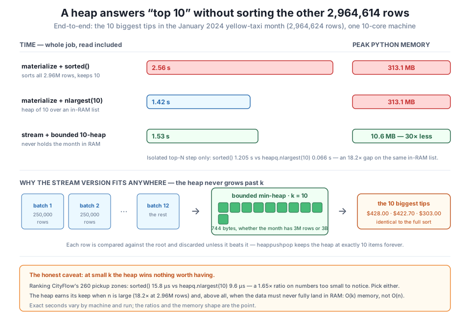
nlargest on a materialized list: 1.42 s but still 313.1 MB, because the O(k) algorithm was handed an O(n) list; the top-N step itself is 18.2× faster (1.205 s → 0.066 s). Bounded 10-heap over Module 4's stream: 1.53 s — marginally slower, since its comparison loop runs in Python rather than C — but only 10.6 MB, a 30× reduction, and the heap itself is just 744 bytes no matter how much data flows past. The remaining 10.6 MB is the 250,000-row batch buffer, so batch_size sets the footprint, not the dataset size. The honest caveat, bottom: on CityFlow's 260 zones the heap saves 6 µs (15.8 vs 9.6 µs, 1.65×) and choosing either is fine. Heaps are about large n and bounded memory, not about small rankings. Exact seconds vary by machine and run; the ratios are the point.The bounded-heap pattern, in one shape
This is the pattern worth memorising, because it composes with everything in Modules 4 and 5: keep a heap of exactly k, compare each arriving row against heap[0], and discard it if it loses. The guard elif tip > heap[0][0] matters — checking the root before calling heappushpop skips the tuple construction and the sift for the ~99.99% of rows that will never make the top ten. Because the state is O(k) and fixed, each worker in a multiprocessing.Pool can keep its own k-heap over its own partition and return just k items; merging p partial answers is then heapq.nlargest(k, chain(*partials)) over p×k rows. Top-N is trivially parallel, and the reduce step is tiny.
A heap and a priority queue are the same object seen from two angles. If instead of (count, zone) you push (priority, task), then “give me the smallest” becomes “give me the most urgent job,” and you have a work scheduler. CityFlow’s nightly pipeline has exactly this need: a dashboard refresh must run before a warehouse vacuum, and an outage alert before either.
work = []
for priority, task in [(2, "backfill January"), (1, "refresh dashboard"),
                       (3, "vacuum warehouse"), (1, "alert on outage")]:
    heapq.heappush(work, (priority, task))

print("draining the queue in priority order:")
while work:
    priority, task = heapq.heappop(work)
    print(f"  priority {priority}: {task}")
draining the queue in priority order:
priority 1: alert on outage
priority 1: refresh dashboard
priority 2: backfill January
priority 3: vacuum warehousePriority 1 jobs first, then 2, then 3, regardless of push order. But look closely at the two priority-1 jobs: "alert on outage" came out before "refresh dashboard" even though it was pushed last. When the priorities tied, Python fell through to comparing the second element — the strings — and "alert on outage" < "refresh dashboard" alphabetically. The queue silently ordered by task name. That is harmless here and a nasty surprise elsewhere, and it is a hint about what happens when the second element cannot be compared at all. Swap the string for a realistic job object:
class Job:
    def __init__(self, name):
        self.name = name
    def __repr__(self):
        return f"Job({self.name!r})"

fragile = []
heapq.heappush(fragile, (1, Job("refresh dashboard")))
print("first push succeeds :", fragile[0])
try:
    heapq.heappush(fragile, (1, Job("alert on outage")))
    print("second push succeeded")
except TypeError as err:
    print("second push raises  : TypeError:", err)
first push succeeds : (1, Job('refresh dashboard'))
second push raises : TypeError: '<' not supported between instances of 'Job' and 'Job'There it is: TypeError: '<' not supported between instances of 'Job' and 'Job'. This trap is genuinely mean, and the printout shows exactly why. The first push succeeded — a one-item heap compares nothing. The failure only appears on the second push, and only because both jobs happened to have priority 1: had they been 1 and 2, the integers would have settled it and Job.__lt__ would never have been reached. A queue like this can run correctly for months and then crash at 3 a.m. the first night two jobs are filed at the same priority. The comparison is data-dependent, so tests that only use distinct priorities will never catch it.
The fix is a monotonically increasing sequence number wedged between the priority and the payload. Ties in priority are then broken by the counter, which is always unique and always orderable — so the comparison never reaches the third element:
tie_breaker = count()
robust = []
for priority, task in [(2, "backfill January"), (1, "refresh dashboard"),
                       (1, "alert on outage"), (1, "rebuild index")]:
    heapq.heappush(robust, (priority, next(tie_breaker), Job(task)))

print("draining with a sequence number as tie-breaker:")
while robust:
    priority, seq, job = heapq.heappop(robust)
    print(f"  priority {priority} (seq {seq}): {job}")
draining with a sequence number as tie-breaker:
priority 1 (seq 1): Job('refresh dashboard')
priority 1 (seq 2): Job('alert on outage')
priority 1 (seq 3): Job('rebuild index')
priority 2 (seq 0): Job('backfill January')No TypeError, and a bonus worth having: the three priority-1 jobs now emerge in seq order 1, 2, 3 — the order they were submitted. The counter has made the queue stable (first-come-first-served within a priority), which is almost always the behaviour a scheduler should have, and it is strictly better than the accidental alphabetical ordering from the string version. itertools.count() is the idiomatic source: it never repeats and never runs out.
Always put a tie-breaker in a priority queue
Push (priority, next(counter), payload), never (priority, payload), unless you are certain the payload is orderable and you want ties broken by its value. The three-tuple costs nothing, removes a TypeError that only fires on tied priorities, and buys stable first-in-first-out ordering within each priority level for free. If the payload is a dict, a custom object, or anything without __lt__, the counter is not a nicety — it is the only thing standing between you and a crash on the first tie.
Everything so far leaned on heap[0] being the smallest, because heapq implements a min-heap and offers no max=True switch. Yet nearly every dashboard question — busiest, biggest, longest — wants the largest. There are three ways across the gap, and they are not equally good:
three = [(145240, "JFK Airport"), (20197, "SoHo"), (143471, "Midtown Center")]

as_min = list(three)
heapq.heapify(as_min)
print("min-heap root (smallest) :", as_min[0])

negated = [(-n, name) for n, name in three]
heapq.heapify(negated)
n, name = negated[0]
print("negated root (largest)   :", (-n, name))
print("nlargest(1) does it too  :", heapq.nlargest(1, three))
min-heap root (smallest) : (20197, 'SoHo')
negated root (largest) : (145240, 'JFK Airport')
nlargest(1) does it too : [(145240, 'JFK Airport')]Negation flips the order: the largest count has the most negative key, so it sorts smallest and lands on the root — just remember to negate back on the way out, and note it only works on numbers (you cannot negate a zone name). heapq.nlargest / nsmallest hide the whole issue and are what you should reach for by default when the data is already in memory.
The third way is the one used in the streaming section, and it is worth naming because it is the least obvious: for a bounded top-N heap, a min-heap is not a workaround at all — it is precisely the right tool. To keep the ten largest items you need instant access to the smallest of your current best ten, since that is the one a new contender must beat and the one to evict. heap[0] gives you exactly that in O(1). A max-heap would put the wrong end at the root and make eviction a linear scan. Python’s “limitation” is what makes the pattern work.
Exercise 1 — Find the crossover. The lesson measured sorted() against heapq.nlargest(10, ...) at n = 260 (a 1.65x ratio, not worth having) and at n = 2,964,624 (18.2x, very much worth having). Somewhere between those lies the size where the heap starts to matter. Take the tips list of real trips and, for n in 1,000 / 10,000 / 100,000 / 1,000,000, time both approaches on tips[:n] and print the ratio for each. Then hold n fixed at 1,000,000 and sweep k over 1 / 10 / 100 / 10,000 / 100,000, timing nlargest(k, ...) each time. Where does the heap’s advantage disappear, and why does that follow from O(n log k)?
Hint
Rebuild tips first — the lesson deleted it before the streaming section. Repeat the small-n timings enough times to get a stable reading, as the 2000-repeat loop did. For the k sweep, remember that log k grows toward log n as k grows toward n: once k is a large fraction of n, nlargest is maintaining a heap nearly as big as the data and has to sort it at the end anyway, so it should lose to sorted, which is a single highly optimised C routine. Finding the k where it flips is the exercise.
Exercise 2 — Bounded top-N over a bigger key space. The 260-zone key space was too small to reward a heap. Widen it: stream the month once and count trips per (pickup zone, hour-of-day) pair rather than per zone, giving up to 260 × 24 keys. Then report the 15 busiest (zone, hour) combinations. Do it twice — once with sorted(...)[:15] over all the pairs and once with heapq.nlargest(15, ...) — and compare the times against the 1.65x you measured on plain zones. Does a bigger key space move the ratio?
Hint
Add tpep_pickup_datetime to the columns= list in iter_batches, and get the hour from the Arrow column with batch.column("tpep_pickup_datetime").to_pandas().dt.hour. Key the Counter on the tuple (zone_id, hour) and Counter.update on a list of those tuples. Build the (count, zone_name, hour) triples afterwards so the count sorts first. Expect a few thousand distinct keys — enough to move the ratio a little, nowhere near the 18.2x of three million rows. That negative-ish result is the point: report what you measure.
Exercise 3 — A stable priority queue for the nightly pipeline. Build a small TaskQueue class wrapping a heap, with add(priority, job) and pop() methods, where job is a Job instance (no __lt__). Use an itertools.count() tie-breaker internally so that jobs of equal priority come out in submission order. Prove both properties: add at least six jobs with several tied priorities and show the drain order is correct, then demonstrate that the naive (priority, job) version raises TypeError on the same input while yours does not.
Hint
Store the counter as an instance attribute (self._seq = count()) so each queue has its own, and push (priority, next(self._seq), job). Have pop() unpack all three and return only the job, so the sequence number stays a private implementation detail. For the negative half of the proof, wrap the naive pushes in try/except TypeError and print the message — and remember the failure needs two jobs at the same priority, since a one-item heap never compares anything.
You learned the structure that answers “top N” without ordering everything else. A heap is a binary tree flattened into a plain Python list, holding one invariant — every parent \( \leq \) its children — so the minimum is always at index 0 and nothing else is promised; the real heapified printout proved it, coming back with is the list sorted? False and every parent <= its children? True in the same breath. heapq gives you heappush and heappop at \( O(\log n) \), heapify at O(n) (3.3x faster than a million individual pushes on the same data), and heappushpop for the bounded case. You then measured the technique honestly instead of assuming it: on CityFlow’s 260 zones a full sort took 15.8 µs against nlargest’s 9.6 µs — a 1.65x ratio worth nothing, and sorted() is a perfectly good answer there. Scaled to the ten biggest tips among 2,964,624 trips, the same pair of calls split to 1.205 s versus 0.066 s, 18.2x. The deeper win was memory: a bounded 10-heap streamed over Module 4’s batches produced a byte-identical answer in 10.6 MB instead of 313.1 MB (30x) — the heap itself just 744 bytes regardless of input size — at a cost of 0.11 s against in-memory nlargest (1.53 s vs 1.42 s end to end). Finally, a heap of (priority, item) tuples is a priority queue, whose tie-break trap you saw raise a real TypeError: '<' not supported between instances of 'Job' and 'Job' on the second push, fixed by an itertools.count() sequence number that also makes the queue stable.
heap[0], the minimum, is guaranteed; a heap is not a sorted list, and siblings are unordered.heapify is O(n) — sifting down from the middle costs less than n pushes at \( \log n \) each, because the expensive top-of-tree nodes are rare and half the nodes are cost-free leaves. If the data is already a list, heapify it (3.3x measured) rather than pushing in a loop.heappushpop with a heap[0] guard holds exactly k items forever, answering top-N in O(k) memory on data that never fits in RAM (744 bytes of heap, 10.6 MB peak vs 313.1 MB). The peak is set by batch_size, not by dataset size.(priority, next(counter), payload), never (priority, payload). Tied priorities fall through to comparing payloads, which silently reorders orderable ones and raises TypeError on the rest; a counter prevents both and makes the queue stable.CityFlow’s dashboard is made almost entirely of top-N panels — busiest zones, longest trips, biggest fares, worst delays — and this lesson is really about what an engineer does with that observation. The naive instinct is to apply the heap everywhere, and the measurements say that would be silly: on 260 zones you would add an import and a concept to save six microseconds. The opposite instinct, “it’s only a sort, ship it,” is what puts a sorted() over three million rows in a nightly job and quietly costs a second every run, or worse, a list(zip(...)) that allocates 313 MB and dies the month the data doubles. The judgment being trained here is reading \( n \) and \( k \) before choosing, and knowing that time and memory are different questions with different answers — nlargest won on speed while the streamed heap won on footprint, and only one of them still runs when the data outgrows the box. That last point is the thread back through the whole course: Module 4 taught you to stream so data never has to fit, Module 5 taught you to spread work over cores, and the bounded heap is what makes a top-N question answerable inside those constraints — O(k) state per worker, k items back from each, merged in microseconds.
Three lessons in, you have collected a dict for O(1) lookup, a deque for O(1) ends, and now a heap for O(1) access to an extreme — each one fast at a different thing, and each one measured on the same taxi month rather than taken on faith. Lesson 4, Choosing the Right Structure, is where those stop being three separate tools and become one decision. You’ll put dict, list, set, deque, and heap side by side against the operations a pipeline actually performs — lookup, insert, delete, dedup, ordered scan, top-N — measure them on real data, and find the crossover points where the theoretical answer and the measured answer part company, exactly as they did here at 260 zones. The output is a decision guide you can apply before writing the code instead of profiling after it, and it turns the habit this lesson practised — check n and k, then choose — into something you can do in seconds at design time.
Keep DATATWEETS free. Help fund practical data, AI, and engineering lessons for learners worldwide.
