Lesson 4 - Choosing the Right Structure

Welcome to Choosing the Right Structure#

Three lessons in, CityFlow’s toolbox is full. Lesson 1 showed that hashing makes a dict find a zone by id in constant time while a list hunts for it, and that a set answers “have I seen this trip?” the same way. Lesson 2 showed that a deque gives a streaming buffer a genuinely cheap front, where list.pop(0) quietly re-copies every element behind it. Lesson 3 showed that a heap hands you the ten busiest zones without ever sorting the other two hundred and fifty-five. Four structures, four convincing demos — and one problem: knowing what each one does is not the same as knowing which one to reach for on a Tuesday afternoon when the dashboard is slow and a teammate asks whether the zone join should be indexed.

That is the gap this lesson closes, and it closes it by replacing the wrong question with the right one. The wrong question is “which structure is fastest?” — it has no answer, because a structure that is slow to build but instant to query wins overwhelmingly if you query it a million times and loses if you query it twice. The right question is “what is my access pattern, and how often do I perform it?” This lesson proves that with three measurements on 2,964,624 real January 2024 trips: a full comparison matrix of five structures across the seven operations a pipeline actually performs, the crossover point where building a dict index stops costing more than it saves (it lands at about five questions), and the memory bill that speed is paid for in. By the end you’ll have a decision procedure, not a pile of facts.

By the end of this lesson, you will be able to:

• Read Big-O as a practical forecast — what actually happens to the clock when the data gets 10x bigger
• Measure list, dict, set, deque, and heap across lookup, membership, append, pop-front, insert-in-middle, dedup, and top-N, and read where the measurement agrees with the theory and where it does not
• Compute the crossover point for an index — the number of queries at which building it pays for itself — and use it to answer “should I index this?” with a number
• Account for the memory an index costs per element, and tell when an index is not an optimization at all
• Choose a structure from the access pattern rather than from habit or reputation

You’ll need pyarrow and Python’s standard library. Let’s turn four structures into one decision.

The Data#

Everything below runs on CityFlow’s real month: January 2024 yellow-taxi trips from the NYC TLC Trip Record Data page. Fetch it once and save it next to your script; every runnable block reads the local copy by name.

# gate: skip
# One month of real NYC yellow-taxi trips, fetched once from the public TLC site.
import urllib.request
urllib.request.urlretrieve(
    "https://d37ci6vzurychx.cloudfront.net/trip-data/yellow_tripdata_2024-01.parquet",
    "yellow_tripdata_2024-01.parquet",
)

We’ll reduce each trip to the four fields these comparisons need: a trip_id (its position in the month), the pickup and dropoff zone ids, and the distance in miles. Keeping the records as plain tuples means every structure below holds the same objects — so when we compare memory later, we’re comparing the containers, not the contents.

import warnings
warnings.filterwarnings("ignore")
import time, sys, random, heapq, bisect, itertools
from collections import deque, Counter
import pyarrow.parquet as pq

table = pq.read_table(
    "yellow_tripdata_2024-01.parquet",
    columns=["PULocationID", "DOLocationID", "trip_distance"],
)
pickup = table["PULocationID"].to_pylist()
dropoff = table["DOLocationID"].to_pylist()
distance = table["trip_distance"].to_pylist()
del table

N = len(pickup)
trips = [(i, pickup[i], dropoff[i], distance[i]) for i in range(N)]

print(f"trips loaded      : {N:,}")
print(f"one trip record   : {trips[0]}  (trip_id, pickup_zone, dropoff_zone, miles)")
print(f"distinct OD pairs : {len(set(zip(pickup, dropoff))):,}")

trips loaded      : 2,964,624
one trip record   : (0, 186, 79, 1.72)  (trip_id, pickup_zone, dropoff_zone, miles)
distinct OD pairs : 26,335

Just under three million trips, and — a number worth holding onto — only 26,335 distinct origin-destination pairs among them. Roughly 265 zones squared is about 70,000 possible pairs, so the taxi network actually uses about a third of them. That ratio between “rows” and “distinct things” is going to decide more than one result below.

Big-O Is a Forecast, Not a Grade#

Big-O notation has a reputation for being an interview ritual. It is not. It is the single most practical tool in this module, because it answers the only question that matters when your data is growing: if this dataset gets 10x bigger, what happens to my clock? That’s it. Big-O describes how the cost of an operation grows with the size of the collection, written $n$. It deliberately ignores constant factors — it will not tell you whether something takes 3 nanoseconds or 30 — because when $n$ is heading for millions, the shape of the growth swamps the constants.

Here are the five shapes you’ll meet in data work, each phrased as what happens at 10x:

• $O(1)$ — constant. 10x the data, same time. A dict lookup doesn’t care whether the dict holds ten entries or ten million; hashing jumps straight to the slot. This is the only shape that is genuinely free as you scale.
• $O(\log n)$ — logarithmic. 10x the data, a tiny bit slower — you add a constant few steps, not a multiple. Binary search on a sorted list, or a heap push. For practical purposes this is nearly as good as constant.
• $O(n)$ — linear. 10x the data, 10x the time. Scanning a list to find something. Perfectly fine once; ruinous in a loop.
• $O(n \log n)$ — linearithmic. 10x the data, a bit more than 10x — call it 12x. This is what a full sort costs, and it is the practical floor for “put everything in order.”
• $O(n^2)$ — quadratic. 10x the data, 100x the time. This is the shape that turns a script that ran fine on your test file into one that never finishes on the real one.

Those are the claims. Let’s check them against a clock rather than trusting them. We’ll take the same four operations at three sizes, each 10x the last — about 30 thousand trips, about 300 thousand, and the full 2.96 million — and watch what each one does:

def timed(fn, reps):
    """Average seconds per call over `reps` calls."""
    t0 = time.perf_counter()
    for _ in range(reps):
        fn()
    return (time.perf_counter() - t0) / reps

random.seed(11)
sizes = (29_646, 296_462, 2_964_624)
growth = {}

header = f"{'n':>10} {'O(1) dict':>12} {'O(log n) bisect':>17} {'O(n) list scan':>16} {'O(n log n) sort':>17}"
print(header)
print("-" * len(header))
for n in sizes:
    ids = [t[0] for t in trips[:n]]
    index = {t[0]: t for t in trips[:n]}
    ordered = sorted(ids)
    probes = itertools.cycle([random.randrange(n) for _ in range(200)])
    t_dict = timed(lambda: index[next(probes)], 200_000)
    t_bis = timed(lambda: bisect.bisect_left(ordered, next(probes)), 200_000)
    t_scan = timed(lambda: next(probes) in ids, 5 if n > 500_000 else 50)
    t_sort = timed(lambda: sorted(ids), 3)
    growth[n] = (t_dict, t_bis, t_scan, t_sort)
    print(f"{n:>10,} {t_dict*1e6:>10.4f}us {t_bis*1e6:>15.4f}us {t_scan*1e6:>14.1f}us {t_sort*1e3:>15.1f}ms")
    del ids, index, ordered
print("-" * len(header))
print("what one step of 10x more data costs:")
for j, label in enumerate(("O(1) dict", "O(log n) bisect", "O(n) list scan", "O(n log n) sort")):
    f1 = growth[sizes[1]][j] / growth[sizes[0]][j]
    f2 = growth[sizes[2]][j] / growth[sizes[1]][j]
    print(f"  {label:<16} {f1:>6.2f}x  then {f2:>6.2f}x")

         n    O(1) dict   O(log n) bisect   O(n) list scan   O(n log n) sort
----------------------------------------------------------------------------
    29,646     0.0450us          0.1881us           71.5us             0.1ms
   296,462     0.0478us          0.2333us          663.7us             1.3ms
 2,964,624     0.0460us          0.2919us         8754.8us            20.2ms
----------------------------------------------------------------------------
what one step of 10x more data costs:
  O(1) dict          1.06x  then   0.96x
  O(log n) bisect    1.24x  then   1.25x
  O(n) list scan     9.29x  then  13.19x
  O(n log n) sort   10.06x  then  16.12x

Read that table as a set of predictions being kept and broken. The dict is flat: 0.0450 µs at thirty thousand trips, 0.0460 µs at three million. A hundredfold more data and the lookup time did not move (1.06x then 0.96x — that’s measurement noise around 1.00x, and the 0.96x is a reminder that noise cuts both ways). That is $O(1)$ doing exactly what it says.

Bisect barely moves: 1.24x then 1.25x per 10x of data. That’s $O(\log n)$ behaving, and you can check the theory arithmetic yourself — going from $n$ = 29,646 to $n$ = 296,462 takes $\log_2 n$ from about 14.9 to about 18.2, a ratio of 1.22. We measured 1.24. Theory and clock agree to within a rounding error.

The list scan tracks 10x, then overshoots: 9.29x, then 13.19x. The first step is textbook $O(n)$. The second is worse than linear, and the honest thing to do is say so and explain it rather than round it into the story. Big-O counts operations; it does not know about hardware. At 30 thousand entries the list of pointers fits comfortably in the CPU’s cache and each step is nearly free; at 2.96 million it does not, so every step of the scan is a trip to main memory. Same $O(n)$ algorithm, worse constant, because the constant was never really constant. The same effect inflates the sort’s second step to 16.12x against a predicted ~12x.

This is the most important caveat about Big-O, so let’s state it plainly: Big-O predicts the shape, not the number. It told us the scan would get dramatically worse and the dict would not, and it was completely right about that. It did not tell us the scan would degrade by 13.19x rather than 10x, because that part is cache physics. Use Big-O to choose the algorithm; use a clock to know your actual cost.

The Measured Comparison Matrix#

Theory settled, here is the table this lesson exists for. Five structures — list, dict, set, deque, and a heap — measured across the operations a real pipeline performs, all holding the same 2.96 million trip records. The benchmark works on copies where an operation mutates, so every structure faces the same collection.

Two notes on reading it before the numbers land. First, n/a is not a missing measurement — it means the structure cannot do that operation at all, and those gaps are as informative as the timings. A set has no “lookup by key” because it stores no values; a dict has no “pop front” because it has no front to pop. Choosing a structure is as much about capability as speed. Second, the units shift per cell (ns, µs, ms) precisely because the spread is so enormous that a single unit would be unreadable.

probes = itertools.cycle([random.randrange(N) for _ in range(200)])

trip_ids   = [t[0] for t in trips]
trip_dict  = {t[0]: t for t in trips}
id_set     = set(trip_ids)
trip_deque = deque(trips)
trip_heap  = [(t[3], t[0]) for t in trips]
heapq.heapify(trip_heap)

bench_list  = list(trips)          # copies: the matrix mutates them
bench_deque = deque(trips)
bench_heap  = list(trip_heap)
rec = trips[0]

def scan_by_key():
    k = next(probes)
    for t in trips:
        if t[0] == k:
            return t

matrix = {}
matrix["lookup by key"] = {
    "list": timed(scan_by_key, 10),
    "dict": timed(lambda: trip_dict[next(probes)], 200_000),
    "set": None, "deque": None, "heap": None,
}
matrix["membership test"] = {
    "list": timed(lambda: next(probes) in trip_ids, 10),
    "dict": timed(lambda: next(probes) in trip_dict, 200_000),
    "set": timed(lambda: next(probes) in id_set, 200_000),
    "deque": None, "heap": None,
}
matrix["append one"] = {
    "list": timed(lambda: bench_list.append(rec), 200_000),
    "dict": timed(lambda: trip_dict.__setitem__(-1, rec), 200_000),
    "set": timed(lambda: id_set.add(-1), 200_000),
    "deque": timed(lambda: bench_deque.append(rec), 200_000),
    "heap": timed(lambda: heapq.heappush(bench_heap, (0.0, -1)), 200_000),
}
matrix["pop front / min"] = {
    "list": timed(lambda: bench_list.pop(0), 2_000),
    "dict": None, "set": None,
    "deque": timed(lambda: bench_deque.popleft(), 200_000),
    "heap": timed(lambda: heapq.heappop(bench_heap), 200_000),
}
matrix["insert in middle"] = {
    "list": timed(lambda: bench_list.insert(len(bench_list)//2, rec), 2_000),
    "dict": None, "set": None,
    "deque": timed(lambda: bench_deque.insert(len(bench_deque)//2, rec), 2_000),
    "heap": None,
}

def fmt(v):
    if v is None:
        return "n/a"
    if v < 1e-6:
        return f"{v*1e9:.0f} ns"
    if v < 1e-3:
        return f"{v*1e6:.1f} us"
    return f"{v*1e3:.2f} ms"

cols = ("list", "dict", "set", "deque", "heap")
head = f"{'operation':<20}" + "".join(f"{c:>13}" for c in cols)
print(head)
print("-" * len(head))
for op, row in matrix.items():
    print(f"{op:<20}" + "".join(f"{fmt(row[c]):>13}" for c in cols))
print("-" * len(head))
print(f"lookup by key   : list / dict  = {matrix['lookup by key']['list']/matrix['lookup by key']['dict']:>9,.0f}x")
print(f"membership test : list / set   = {matrix['membership test']['list']/matrix['membership test']['set']:>9,.0f}x")
print(f"pop front       : list / deque = {matrix['pop front / min']['list']/matrix['pop front / min']['deque']:>9,.0f}x")
print(f"insert middle   : deque / list = {matrix['insert in middle']['deque']/matrix['insert in middle']['list']:>9.2f}x")

del bench_list, bench_deque, bench_heap

operation                    list         dict          set        deque         heap
-------------------------------------------------------------------------------------
lookup by key            24.89 ms        47 ns          n/a          n/a          n/a
membership test           6.74 ms        45 ns        42 ns          n/a          n/a
append one                  31 ns        70 ns        31 ns        32 ns        85 ns
pop front / min          466.9 us          n/a          n/a        30 ns       395 ns
insert in middle         751.7 us          n/a          n/a      1.05 ms          n/a
-------------------------------------------------------------------------------------
lookup by key   : list / dict  =   526,222x
membership test : list / set   =   159,814x
pop front       : list / deque =    15,603x
insert middle   : deque / list =      1.40x

Now put the theory next to the clock, row by row.

Lookup by key — theory says $O(n)$ for a list, $O(1)$ for a dict. Measured: 24.89 ms against 47 ns, a factor of 526,222. Theory and measurement agree completely, and the size of the gap is the reason this module exists. Note this is a short-circuiting scan — it stops when it finds the key, so on average it only walks half the list — and it still loses by five and a half orders of magnitude.

Membership test — same shapes, same verdict: 6.74 ms against a set’s 42 ns, 159,814x. Two details reward a second look. The list membership test (6.74 ms) is much faster than the list key-lookup (24.89 ms) even though both are $O(n)$ scans, because in on a list of plain ints compares integers in C, while scan_by_key runs a Python-level loop and unpacks a tuple field per row. Identical Big-O, ~4x different constant — exactly the sort of thing Big-O is designed not to tell you. And set (42 ns) edges out dict (45 ns), which makes sense: both hash the key, but the set has no value to fetch.

Append one — everything is fast and everything is flat. list 31 ns, set 31 ns, deque 32 ns, dict 70 ns, heap 85 ns. The heap is the only $O(\log n)$ entry here, and $\log_2$ of 2.96 million is only about 21 — so “logarithmic” costs it 85 ns against a list’s 31. The lesson: when everything is $O(1)$-ish, the choice does not matter; stop optimizing and pick on capability instead.

Pop front — the trap Lesson 2 named, now sized: list.pop(0) takes 466.9 µs while deque.popleft() takes 30 ns. That’s 15,603x, and it is pure $O(n)$ versus $O(1)$: popping a list’s first element shifts all 2.96 million remaining pointers down one slot. The heap’s 395 ns is a different operation — it pops the minimum, not the front — and it is $O(\log n)$, which again costs almost nothing in absolute terms.

Insert in the middle — and here is the row that contradicts the naive expectation, which is why it’s the most instructive one in the table. A list is famously the “array” structure and a deque is famously the “fast insert” structure, so you might expect the deque to win. It loses: 1.05 ms against the list’s 751.7 µs, a full 1.40x slower. Both are $O(n)$, so Big-O calls it a tie and the constants break it. A list stores its pointers in one contiguous block, so inserting in the middle is a single memmove — bulk hardware work the CPU is exceptionally good at. A deque stores its elements in a chain of fixed-size blocks, so inserting in the middle means walking the chain and rotating elements through it, in slower per-element steps. The deque’s $O(1)$ superpower is at the ends, and only at the ends. Reach for it in the middle and you get the worst of both.

The general reading of the table: the gaps that matter are orders of magnitude, and they all come from picking a structure whose cheap operations match what you actually do. The gaps that don’t matter — 31 ns vs 32 ns on append — are noise you should never spend a decision on.

Dedup and Top-N: Where the Shape Becomes the Story#

Two whole-collection operations from Lessons 1 and 3 round out the matrix, and they need their own section because they show growth rather than a single cost.

Deduplicating by scanning — the “check if I’ve seen it, in a list” approach that feels natural before you know better — is the $O(n^2)$-shaped operation we couldn’t fit in the growth table. Here it is at sizes that finish, alongside a set doing the same job:

od_pairs = list(zip(pickup, dropoff))

def dedup_by_scanning(seq):
    seen = []
    for x in seq:
        if x not in seen:
            seen.append(x)
    return seen

print(f"{'n':>8} {'distinct':>10} {'list dedup':>13} {'growth':>8} {'set dedup':>13} {'growth':>8}")
print("-" * 66)
prev_l = prev_s = None
last_n = last_distinct = 0
for n in (5_000, 10_000, 20_000, 40_000):
    chunk = od_pairs[:n]
    t0 = time.perf_counter(); got_l = dedup_by_scanning(chunk); s_l = time.perf_counter() - t0
    got_s = set(chunk)
    s_s = timed(lambda: set(chunk), 50)   # sub-ms: average many runs
    g_l = "-" if prev_l is None else f"{s_l/prev_l:.2f}x"
    g_s = "-" if prev_s is None else f"{s_s/prev_s:.2f}x"
    print(f"{n:>8,} {len(got_l):>10,} {s_l*1e3:>10.1f} ms {g_l:>8} {s_s*1e3:>10.3f} ms {g_s:>8}")
    prev_l, prev_s = s_l, s_s
    last_n, last_distinct = n, len(got_l)
print("-" * 66)

t0 = time.perf_counter(); unique_set = set(od_pairs); s_set = time.perf_counter() - t0
t0 = time.perf_counter(); unique_dict = dict.fromkeys(od_pairs); s_dict = time.perf_counter() - t0
print(f"dedup all {N:,} OD pairs with set()          : {s_set*1e3:7.1f} ms -> {len(unique_set):,} unique")
print(f"dedup all {N:,} OD pairs with dict.fromkeys(): {s_dict*1e3:7.1f} ms -> {len(unique_dict):,} unique")

# list dedup does roughly n * (distinct/2) comparisons; scale the last measured run up
work_measured = last_n * (last_distinct / 2)
work_full = N * (len(unique_set) / 2)
projected = prev_l * (work_full / work_measured)
print(f"projected list-scan dedup at {N:,} rows       : {projected:7.0f} s  ({projected/60:.1f} min)")
print(f"                                    set is    : {projected/s_set:7,.0f}x faster")

ranked = list(zip(distance, range(N)))
t0 = time.perf_counter(); by_sort = sorted(ranked, reverse=True)[:10]; s_sort = time.perf_counter() - t0
t0 = time.perf_counter(); by_heap = heapq.nlargest(10, ranked); s_heap = time.perf_counter() - t0
print(f"top-10 longest trips, sorted()[:10]      : {s_sort*1e3:7.1f} ms")
print(f"top-10 longest trips, heapq.nlargest(10) : {s_heap*1e3:7.1f} ms  ({s_sort/s_heap:.1f}x faster)")
print(f"same answer: {by_sort == by_heap}")

del od_pairs, unique_dict, ranked

       n   distinct    list dedup   growth     set dedup   growth
------------------------------------------------------------------
   5,000      1,970       34.7 ms        -      0.127 ms        -
  10,000      2,867       90.4 ms    2.61x      0.248 ms    1.95x
  20,000      4,159      232.7 ms    2.57x      0.489 ms    1.97x
  40,000      5,689      646.5 ms    2.78x      0.973 ms    1.99x
------------------------------------------------------------------
dedup all 2,964,624 OD pairs with set()          :    65.0 ms -> 26,335 unique
dedup all 2,964,624 OD pairs with dict.fromkeys():    79.6 ms -> 26,335 unique
projected list-scan dedup at 2,964,624 rows       :     222 s  (3.7 min)
                                    set is    :   3,415x faster
top-10 longest trips, sorted()[:10]      :   766.9 ms
top-10 longest trips, heapq.nlargest(10) :    60.7 ms  (12.6x faster)
same answer: True

The set column is a clean $O(n)$: 1.95x, 1.97x, 1.99x per doubling of the data. Textbook.

The list column is where honesty is required. Every doubling roughly 2.6x to 2.8xes the time — and if list-scan dedup were truly $O(n^2)$, doubling $n$ would quadruple it. We measured 2.6x, not 4x. The measurement contradicts the textbook label, and the explanation is the number we flagged at the start: the inner x not in seen scans the list of distinct items found so far, not all $n$ items. Distinct grows sublinearly here — 1,970 → 2,867 → 4,159 → 5,689 as $n$ doubles — because taxi trips reuse the same routes. So the true cost is $O(n \cdot d)$ where $d$ is the distinct count, and only when every element is unique ($d = n$) does that collapse to the $O(n^2)$ worst case. Real data is kinder than the worst case. This is exactly why you measure: the label said 4x, the data said 2.6x, and both are correct once you know what $d$ is doing.

Kinder is not kind, though. Scaling that last measured run by $n \cdot d$ projects the list approach at 222 seconds — nearly four minutes — where the set takes 65.0 ms. That’s 3,415x, and it is the gap between a pipeline step you don’t notice and one you go get coffee during. (dict.fromkeys does the same job in 79.6 ms and additionally preserves first-seen order — a set is marginally faster, a dict keeps the order; pick on whether order matters.)

Top-N closes the matrix: heapq.nlargest(10, ...) finds the ten longest trips in 60.7 ms where sorted(...)[:10] needs 766.9 ms — 12.6x — and both return the identical answer. The heap never sorts 2.96 million trips to hand back ten; it keeps ten and streams past the rest, $O(n \log 10)$ against the sort’s $O(n \log n)$.

The Crossover: When Does an Index Pay for Itself?#

Every number so far has quietly cheated. Each one measured the cost of using a structure and ignored the cost of building it — and building is where the whole decision actually lives.

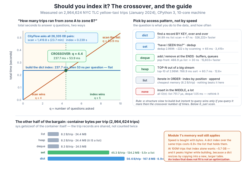
Here is the bargain in its honest form. A list costs nothing to build; the trips already arrive as a sequence. A dict index has to be constructed, which means one full pass over every row before it can answer anything. So for one query, the list wins outright: it starts answering immediately while the dict is still hashing three million rows. For a million queries, the dict wins by a margin so large it’s hard to write down. Somewhere between one and a million is a crossover point — the query count where the two total costs are equal — and that number, not any raw speed, is the answer to “should I index this?”

Let’s find it for a real CityFlow question: “how many trips ran from zone A to zone B?” The list answers by scanning all 2.96 million trips and counting matches — and note this scan cannot short-circuit, because it needs every match, not the first. The dict answers by building a Counter over the OD pairs once, then reading a key.

def count_by_scanning(a, b):
    n = 0
    for _, p, d, _dist in trips:
        if p == a and d == b:
            n += 1
    return n

t0 = time.perf_counter()
od_index = Counter((t[1], t[2]) for t in trips)
build_secs = time.perf_counter() - t0

random.seed(7)
questions = random.sample(sorted(od_index.keys()), 10)
ask = itertools.cycle(questions)
per_scan = timed(lambda: count_by_scanning(*next(ask)), 10)
per_hit = timed(lambda: od_index[next(ask)], 200_000)

print(f"build the OD index once      : {build_secs*1e3:8.1f} ms   ({len(od_index):,} distinct pairs)")
print(f"answer 1 question by scanning: {per_scan*1e3:8.1f} ms")
print(f"answer 1 question from index : {per_hit*1e9:8.1f} ns   ({per_scan/per_hit:,.0f}x faster per question)")

crossover = build_secs / (per_scan - per_hit)
print(f"\ncrossover = build / (scan - hit) = {build_secs*1e3:.1f} ms / ({per_scan*1e3:.1f} ms - {per_hit*1e9:.0f} ns)")
print(f"          = {crossover:.1f} questions\n")

print(f"{'questions':>10} {'scan total':>13} {'index total':>13} {'winner':>10}")
print("-" * 50)
for q in (1, 2, 3, 4, 5, 10, 100, 26_335):
    scan_total = q * per_scan
    index_total = build_secs + q * per_hit
    print(f"{q:>10,} {scan_total:>10.3f} s {index_total:>11.3f} s {'index' if index_total < scan_total else 'scan':>10}")
print("-" * 50)

build the OD index once      :    237.7 ms   (26,335 distinct pairs)
answer 1 question by scanning:     53.9 ms
answer 1 question from index :     53.2 ns   (1,012,777x faster per question)

crossover = build / (scan - hit) = 237.7 ms / (53.9 ms - 53 ns)
          = 4.4 questions

 questions    scan total   index total     winner
--------------------------------------------------
         1      0.054 s       0.238 s       scan
         2      0.108 s       0.238 s       scan
         3      0.162 s       0.238 s       scan
         4      0.216 s       0.238 s       scan
         5      0.270 s       0.238 s      index
        10      0.539 s       0.238 s      index
       100      5.391 s       0.238 s      index
    26,335   1419.840 s       0.239 s      index
--------------------------------------------------

The crossover is 4.4 questions. Under five.

The arithmetic behind it is worth internalising, because it generalises to every indexing decision you will ever make. The two total costs are:

Set them equal and solve for $q$. Since the per-hit term (53.2 ns) is a millionth of the per-scan term and vanishes into rounding, the crossover is essentially just build cost ÷ scan cost: 237.7 ÷ 53.9 = 4.4. In words: the crossover is how many scans it takes to pay for one build. Building the index costs about four and a half scans’ worth of work, so from the fifth question onward it’s free money.

The sweep table shows it exactly where the algebra puts it: at 4 questions the scan is still ahead (0.216 s vs 0.238 s), and at 5 the index takes the lead (0.270 s vs 0.238 s) and never gives it back. Ask all 26,335 OD pairs — which is precisely what a dashboard that renders the full origin-destination matrix does — and scanning needs 1,419.8 seconds, nearly 24 minutes, while the index needs 0.239 seconds. Same answers. About 6,000x.

Now the honest part, twice over. First, 4.4 is not a universal constant — it’s this build against this scan on this machine, and re-running the lesson gives values between roughly 4.4 and 4.8 as the timings jitter. Don’t memorise the digit; memorise the method and the order of magnitude. Second, and more useful: the crossover is small by construction. Building an index is one $O(n)$ pass and answering by scanning is also one $O(n)$ pass, so their ratio can only ever be a small constant — the extra cost of hashing a row versus comparing it. The crossover for a hash index is essentially always a handful, never thousands. That is the quantitative reason “should I index this?” so reliably answers yes: you need to be asking fewer than about five questions for the answer to be no. The genuinely rare case — the one where you should not index — is the one-shot script that answers a single question and exits.

The Other Half of the Bargain: Memory#

Speed is not free — it is bought with bytes, and Module 1’s memory wall never went away. A dict does not conjure constant-time lookups from nothing; it buys them with a sparse hash table that is deliberately kept substantially larger than the number of keys in it, so that hashed keys rarely collide. That empty space is the price of $O(1)$.

We can price it exactly. Because every structure below holds the same trip tuples, sys.getsizeof on the container measures only the container’s own overhead — the records are shared and are not double-counted. That is precisely the number we want: what does the index cost, on top of the data?

def per_element(name, obj, n):
    total = sys.getsizeof(obj)
    print(f"{name:<24}{total:>13,} B{total/n:>12.1f} B/trip")
    return total

print(f"container overhead for {N:,} trips (sys.getsizeof, elements shared & excluded)")
print("-" * 62)
b_list  = per_element("list of trips", trips, N)
b_deque = per_element("deque of trips", trip_deque, N)
b_heap  = per_element("heap (a plain list)", trip_heap, N)
b_set   = per_element("set of trip_ids", id_set, N)
b_dict  = per_element("dict trip_id -> trip", trip_dict, N)
print("-" * 62)
print(f"dict index costs {b_dict/b_list:.1f}x a list, set costs {b_set/b_list:.1f}x")
print(f"the index alone adds {(b_dict-b_list)/1e6:.1f} MB on top of the {b_list/1e6:.1f} MB list")
print(f"at 100,000,000 trips that dict would want ~{b_dict/N*100e6/1e9:.1f} GB of RAM, index only")

print("\nwhy a dict resizes in jumps (and why the peak is worse than the final size):")
d = {}
last = sys.getsizeof(d)
jumps = 0
for i in range(200_000):
    d[i] = None
    cur = sys.getsizeof(d)
    if cur != last:
        if jumps < 4 or i > 150_000:
            print(f"  at {i+1:>7,} keys the table jumped {last:>10,} B -> {cur:>10,} B")
        last = cur
        jumps += 1
print(f"  {jumps} resizes total; each one allocates the new table while the old is still alive")

container overhead for 2,964,624 trips (sys.getsizeof, elements shared & excluded)
--------------------------------------------------------------
list of trips              24,387,832 B         8.2 B/trip
deque of trips             24,458,776 B         8.3 B/trip
heap (a plain list)        24,387,832 B         8.2 B/trip
set of trip_ids           134,217,944 B        45.3 B/trip
dict trip_id -> trip      167,772,248 B        56.6 B/trip
--------------------------------------------------------------
dict index costs 6.9x a list, set costs 5.5x
the index alone adds 143.4 MB on top of the 24.4 MB list
at 100,000,000 trips that dict would want ~5.7 GB of RAM, index only

why a dict resizes in jumps (and why the peak is worse than the final size):
  at       1 keys the table jumped         64 B ->        224 B
  at       6 keys the table jumped        224 B ->        352 B
  at      11 keys the table jumped        352 B ->        632 B
  at      22 keys the table jumped        632 B ->      1,168 B
  at 174,763 keys the table jumped  5,242,960 B -> 10,485,848 B
  17 resizes total; each one allocates the new table while the old is still alive

The sequential structures are nearly free: a list spends 8.2 bytes per trip, which is one 8-byte pointer plus a sliver of growth room. The deque’s 8.3 and the heap’s 8.2 confirm two things worth knowing — a deque costs essentially the same as a list, and a heap is not a separate structure at all; heapq imposes an ordering discipline on a plain list, which is why its row is byte-identical to the list’s.

The hashed structures are where the money goes: a set costs 45.3 bytes per trip (5.5x a list) and a dict 56.6 bytes per trip (6.9x a list). In absolute terms, indexing this month adds 143.4 MB on top of a 24.4 MB list. You are paying roughly seven bytes of RAM for every one byte a list would have used, and 526,222x faster lookups is what you get back. That is usually an excellent trade — but it is a trade, and it has a breaking point. Scale it to 100 million trips (a bit over two years of yellow-taxi data) and the index alone wants about 5.7 GB, before a single trip record is stored. On a 16 GB laptop that is no longer a speedup; it is an OutOfMemoryError with extra steps.

The resize trace explains why the ceiling is even lower than that. A dict’s table grows in jumps, by doubling — 17 of them on the way to 200,000 keys — and each jump allocates a new, larger table and copies every key into it while the old table is still alive. So the peak memory during a build is meaningfully higher than the finished index’s size, as the 5,242,960 → 10,485,848 byte jump shows. An index that just barely fits in RAM will not survive being built.

The Decision Guide#

Put the three measurements together and the decision procedure falls out. Notice that it never begins with “which structure is fastest?” — it begins with what you do to the data, and how many times.

Start with the access pattern. If you find records by a key and do it more than a handful of times, use a dict: 47 ns against 24.89 ms is 526,222x, and the crossover says you only need about five lookups to be ahead. If you ask “have I seen this?” or need to deduplicate, use a set — same hashing, no values to store, and it deduplicated 2.96 million pairs 3,415x faster than scanning could. If you add and remove at the ends — a streaming buffer, a work queue, a sliding window — use a deque, whose 30 ns popleft beats a list’s 466.9 µs by 15,603x. If you want the top N out of a large stream, use a heap: 12.6x faster than a full sort for the same ten answers, and it never holds more than N.

And if you iterate everything in order, index by position, or just append and read back, use a list. This is the guide’s most under-appreciated branch. The list is not the loser of this lesson — it is the cheapest structure in memory (8.2 B/trip against a dict’s 56.6), it appends as fast as anything measured (31 ns), and for a single pass over the data nothing beats it, because the fancy structures all have to be built from it first. Reach for a dict only when you have a reason, and the crossover is how you name that reason.

Two branches end in a warning rather than a structure. If your pattern is inserting in the middle at high volume, none of these five is right — every one of them is $O(n)$ there, and the measurement showed the “obvious” fix is a regression (a deque’s 1.05 ms is 1.40x slower than a list’s 751.7 µs). That pattern is a signal to rethink the design — usually you want a different grain, a sorted structure, or a real database — not a different container. And if the index won’t fit in memory, the branch goes back to Module 4, not to a bigger dict.

Practice Exercises#

Exercise 1 — Find the crossover for the zone dimension. The OD index crossed over at about 4.4 questions on 2.96 million rows. Build the same measurement for a much smaller collection: the 265-row zone table (taxi_zone_lookup.csv, columns LocationID and Borough). Time how long it takes to build a {LocationID: Borough} dict, time one lookup done by scanning the list of rows, and divide to get the crossover. Predict before you run it whether the crossover will be bigger or smaller than 4.4, then explain the result you actually get.

Exercise 2 — Price a smaller index. The memory section showed a dict over 2.96 million trips costs 167.8 MB. But the OD index — the one that answered every question in the crossover section — has only 26,335 keys. Measure sys.getsizeof for both, report the bytes per key for each, and compute how many MB the OD index saves over the per-trip index. Then explain in a comment why aggregating to a coarser grain before indexing is one of the answers in the memory callout.

Exercise 3 — Break the dedup projection. The lesson projected list-scan dedup at 222 seconds on the full month and explained that it grew at 2.6x per doubling rather than the textbook 4x, because the distinct count $d$ grows sublinearly in this data. Test that explanation by removing the effect: dedup a sequence where every element is unique (say list(range(n))) at $n$ = 1,000, 2,000, 4,000, and 8,000, and report the growth factor per doubling. Then explain in a comment why this sequence shows the true $O(n^2)$ shape while the OD pairs did not.

Summary#

You turned four structures into one decision procedure. Big-O is a forecast of what 10x more data does to the clock — $O(1)$ doesn’t move, $O(\log n)$ barely does, $O(n)$ costs 10x, $O(n \log n)$ about 12x, $O(n^2)$ costs 100x — and the measurements confirmed the shapes while honestly breaking the numbers: a dict lookup held at 0.0450 → 0.0460 µs across a hundredfold more data, bisect grew 1.24x per 10x against a predicted 1.22x, but the list scan degraded 13.19x rather than 10x because at 2.96 million elements it no longer fits in cache. Big-O predicts the shape, not the number. The comparison matrix priced every operation on 2,964,624 real trips: dict lookup beat a list scan 526,222x (47 ns vs 24.89 ms), a set membership test beat a list 159,814x, deque.popleft beat list.pop(0) 15,603x (30 ns vs 466.9 µs), a set deduplicated 2.96M OD pairs 3,415x faster than the projected 222-second scan, and heapq.nlargest found the top 10 12.6x faster than a full sort — while append was a 31-vs-32 ns tie nobody should spend a decision on, and a deque’s insert-in-middle came out 1.40x slower than a list’s, because both are $O(n)$ and a contiguous memmove beats a block chain. The number that actually decides things is the crossover: the OD index costs 237.7 ms to build against 53.9 ms per list scan, so it pays for itself after 4.4 questions — scanning wins at 4, the index wins from 5 onward and by 26,335 questions it is 1,419.8 s against 0.238 s. And the bill: a dict costs 56.6 bytes per trip against a list’s 8.2 (6.9x), adding 143.4 MB here and projecting to ~5.7 GB at 100 million trips — so an index that doesn’t fit is not an optimization.

Key Concepts#

• Big-O as a forecast — it answers “what happens at 10x?”, predicting the growth shape while ignoring constants. It correctly called the dict flat and the scan catastrophic; it could not know the scan would degrade 13.19x rather than 10x, because cache behaviour is not in the notation. Choose the algorithm with Big-O, know your cost with a clock.
• Access pattern, not speed — “which structure is fastest?” has no answer. Lookup by key → dict; membership and dedup → set; add/remove at the ends → deque; top-N → heap; iterate in order or index by position → list. The gaps that matter are orders of magnitude; a 31-vs-32 ns append is not a decision.
• The crossover — an index’s build cost divided by one scan’s cost gives the query count at which indexing pays for itself: 237.7 ms ÷ 53.9 ms = 4.4 questions here. Since building and scanning are both one $O(n)$ pass, the ratio is always a small constant — which is why “should I index this?” answers yes unless you truly are asking once.
• Capability before speed — n/a in the matrix means the structure cannot do the operation, not that it is slow. A set has no lookup-by-key, a dict has no front to pop, a heap is a list under an ordering discipline (byte-identical at 8.2 B/trip). Half of choosing well is knowing what a structure refuses to do.
• Speed is bought with bytes — hashing costs a deliberately sparse table: 56.6 B/trip for a dict and 45.3 for a set against 8.2 for a list, plus a resize peak because dicts grow by copying into a doubled table. Multiply bytes-per-element by your element count before indexing; if it doesn’t fit, chunk it, index only keys, or aggregate to a coarser grain.

Why This Matters#

CityFlow’s dashboard renders the full origin-destination matrix — all 26,335 pairs — and on the scanning implementation that is 1,419.8 seconds of work that no amount of Module 5’s parallelism can rescue. Ten cores would take nearly 24 minutes down to a few minutes; the dict takes it to 0.238 seconds on one core. That is the module’s spine in a single comparison: parallelism makes wasteful work finish sooner, while the right structure means the work never happens. But the lesson that outlives any of these numbers is the method. You now answer “should I index this?” the way an engineer does — not with a preference, not with a rule of thumb about dicts being fast, but by timing the build once, timing one query each way, dividing, and getting a number. Then you check that the number’s price in RAM is one you can actually pay. The four structures will still be here in ten years; the habit of turning an architecture argument into a measurement is what makes you the person in the room who can end it.

Continue Building Your Skills#

You have the decision procedure; Lesson 5, the guided project In-Memory Index and Top-N, is where it becomes an artifact. You’ll build the thing every measurement above has been pointing at: a reusable module that makes one pass over the real month of trips and comes back with both a dict index from zone to its trips and a heap-maintained top-N ranking — the two structures filled in a single traversal rather than one pass each, because by then you’ll know exactly why a second pass is 53.9 ms you didn’t need to spend. You’ll measure it against a naive baseline that scans and sorts, and the speedup you see will not be a surprise — you will have predicted it from the crossover, the top-N ratio, and the memory bill you priced here. That is what it feels like when the theory has been measured first: the project stops being a demo and starts being a component you would actually ship.