Lesson 5 - Guided Project: An In-Memory Index + Top-N

Welcome to the Guided Project: An In-Memory Index + Top-N#

Four lessons ago, a dict was a way to look something up. Since then you have measured what that actually buys: a hash lookup that answers in constant time while a list scan slows down with every row, a set that tests membership just as fast, a deque whose front is genuinely O(1) where list.pop(0) quietly re-copies the world, and a heap that hands you the ten largest values out of millions without sorting the rest. Each of those was a measurement on its own. CityFlow’s dashboard team does not want measurements — they want a service. They want to open a page and see the busiest pickup zones in New York last month, by name, with the average fare, plus the handful of eye-watering individual fares that the analysts always ask about.

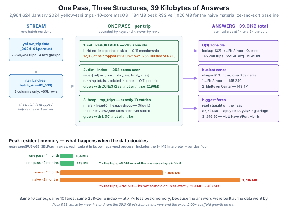
This project builds that service, and it builds it under a constraint that makes the whole module worth learning: one pass over the data, and memory that does not grow with the number of trips. Every answer the dashboard needs gets assembled while the trips stream by — the index, the ranking, and the outliers — and then the source data is thrown away. You will build it in labelled steps, prove it against a naive baseline that materializes and sorts everything, and measure both time and peak memory honestly. The headline is real and measured on this page: the same ten zones and the same ten fares at a 134 MB peak instead of 1,026 MB, and when the input doubles the service grows by 9 MB while the baseline grows by 769. Best of all is the number that ends the lesson: the answers the service actually keeps weigh 39 kilobytes.

By the end of this project, you will be able to:

• Combine a dict index, a set filter, and a bounded heap into a single streaming pass
• Explain why an aggregate top-N comes from nlargest over the finished index, but a per-row top-N needs a heap during the pass
• Measure peak resident memory honestly with getrusage, and say what it does and does not count
• Show that one-pass memory is bounded by keys and k, not by row count, by doubling the input
• Decide against a data structure on evidence, and package the result as a reusable module

You’ll need pyarrow, pandas, and Python’s standard library (heapq, collections, resource, multiprocessing).

The goal and the acceptance criteria#

Before writing code, write down what “done” means. A guided project without acceptance criteria is just typing.

CityFlow’s zone-activity service must, given a month of trip records, produce four things: an index from zone id to that zone’s accumulated statistics (trip count, total fare, total distance) enriched with the human-readable zone and borough name; the top 10 busiest zones by trip count; the top 10 individual trips by fare; and an O(1) lookup so a dashboard tile for any single zone renders without touching the trip data again.

It must satisfy these constraints:

1. One pass. The trip records are read exactly once, in batches. No second scan, no per-zone re-scan.
2. Bounded memory. Peak memory is a function of the number of zones (a few hundred) and the top-N size k (ten) — not the number of trips. Doubling the trips must not double the memory.
3. Correct. The answers must match a dumb, obviously-correct baseline exactly.
4. Honest structures. Every data structure in the final module must earn its place. A structure that does not fit gets removed, not decorated with a comment.
5. Reusable. The result is an importable module, not a script that prints things.

The data is New York City’s public-domain Yellow Taxi trip records, published by the NYC Taxi & Limousine Commission on its Trip Record Data page — the same January 2024 month you have been streaming since Module 4, plus the small zone dimension you joined in Lesson 1:

• Trips: https://d37ci6vzurychx.cloudfront.net/trip-data/yellow_tripdata_2024-01.parquet (2,964,624 rows)
• Zone lookup: https://datatweets.com/datasets/nyc-taxi/taxi_zone_lookup.csv (265 zones)

As always, a real pipeline downloads once and then reads the local cached copy, so every runnable block below reads the bare filenames:

# gate: skip
# Fetch once; every block afterwards reads the local cached copies by name.
import urllib.request
urllib.request.urlretrieve(
    "https://d37ci6vzurychx.cloudfront.net/trip-data/yellow_tripdata_2024-01.parquet",
    "yellow_tripdata_2024-01.parquet")
urllib.request.urlretrieve(
    "https://datatweets.com/datasets/nyc-taxi/taxi_zone_lookup.csv",
    "taxi_zone_lookup.csv")

Step 1: The zone dimension — a dict and a set#

The zone lookup is 265 rows, which is nothing, and that is exactly why it belongs in memory as a dict. Lesson 1 made the case with a stopwatch: finding a zone by id in a dict is constant-time, while scanning a list of 265 zones for every one of 2.96 million trips is 265 comparisons times 2.96 million — the kind of arithmetic that turns a three-second job into a three-minute one. So the dimension is loaded once, up front, into zone_name.

The set is the more interesting half of this step, and it comes from the data itself rather than from a tutorial’s wish to feature a set. The lookup table has 265 entries, but two of them are not real places: id 264 has borough Unknown and no zone name at all, and id 265 is the catch-all Outside of NYC with no borough. A dashboard cannot render a tile for “Unknown”. Those trips must be filtered out, and the filter runs once per trip — 2.96 million times. That is precisely the access pattern a set is for: a membership test that must be O(1) because it happens on the hot path.

import warnings; warnings.filterwarnings("ignore")
import time, sys, heapq, resource
import multiprocessing as mp
from collections import defaultdict, deque
import pandas as pd
import pyarrow.parquet as pq

MONTH = "yellow_tripdata_2024-01.parquet"
COLS = ["PULocationID", "trip_distance", "fare_amount"]

def load_zone_dimension(path="taxi_zone_lookup.csv"):
    """Return (zone_name dict, reportable id set) -- the Lesson 1 structures."""
    z = pd.read_csv(path)
    zone_name = {int(r.LocationID): (r.Zone, r.Borough) for r in z.itertuples()}
    reportable = {int(r.LocationID) for r in z.itertuples()
                  if isinstance(r.Zone, str) and isinstance(r.Borough, str)
                  and r.Borough != "Unknown"}
    return zone_name, reportable

if __name__ == "__main__":
    ZONE_NAME, REPORTABLE = load_zone_dimension()
    print("zone_name dict entries :", len(ZONE_NAME))
    print("reportable id set      :", len(REPORTABLE))
    print("dropped as unreportable:", sorted(set(ZONE_NAME) - REPORTABLE))
    for zid in (132, 161, 264, 265):
        print(f"  {zid} -> {ZONE_NAME[zid]}   reportable={zid in REPORTABLE}")

zone_name dict entries : 265
reportable id set      : 263
dropped as unreportable: [264, 265]
  132 -> ('JFK Airport', 'Queens')   reportable=True
  161 -> ('Midtown Center', 'Manhattan')   reportable=True
  264 -> (nan, 'Unknown')   reportable=False
  265 -> ('Outside of NYC', nan)   reportable=False

Two structures, both tiny, both permanent for the life of the service: a 265-entry dict that turns an id into a name, and a 263-entry set that answers “should this trip be counted?” in constant time. Notice that the set was derived from the data’s own quality problem — the nan zone name on 264 and the nan borough on 265 — rather than hard-coded. When the TLC adds a zone next year, the set adjusts itself.

Step 2: The one-pass core#

Here is the heart of the project, and the shape is worth reading before the code. A single loop pulls batches of 65,536 rows out of the Parquet file with iter_batches, and for each trip inside a batch it does exactly three cheap things: test the zone against the set, update the zone’s running totals in the dict, and offer the fare to the heap. When the batch is done it is dropped and the next one is read. At no point does the whole month exist in memory.

The dict is the index. Its value is a mutable three-slot list — [trips, total_fare, total_miles] — updated in place, because a running total is all you need to compute an average later. This is the distinction that keeps memory flat: the naive instinct is to append every fare to a per-zone list and sum it at the end, which stores 2.96 million floats; running totals store three numbers per zone, forever, no matter how many trips arrive.

The heap is the other half. Lesson 3 established the pattern: keep a min-heap of at most k items, and for each new value, if the heap is full and the value beats the smallest thing in it (heap[0]), heappushpop it in. The heap never exceeds ten entries, so the other 2,952,596 fares are compared once and thrown away, never stored, never sorted.

The deque gets a small, honest job: a rolling throughput monitor with maxlen=8, so a long-running ingest can report a live rows-per-second figure without accumulating a timing list that grows all day. It is bounded by construction — pushing a ninth entry silently drops the first — which is the whole reason to reach for deque(maxlen=...) rather than a list you have to remember to trim.

def build_zone_activity(path, top_k=10, batch_size=65_536, repeats=1):
    """ONE streaming pass: dict index + bounded heap + set filter + deque monitor."""
    zone_name, reportable = load_zone_dimension()
    index = defaultdict(lambda: [0, 0.0, 0.0])   # zone id -> [trips, fare, miles]
    top_trips = []                                # bounded min-heap, len <= top_k
    rates = deque(maxlen=8)                       # rolling throughput, bounded
    seen = skipped = 0

    for _ in range(repeats):
        for batch in pq.ParquetFile(path).iter_batches(batch_size=batch_size, columns=COLS):
            t_batch = time.perf_counter()
            zones = batch.column("PULocationID").to_pylist()
            miles = batch.column("trip_distance").to_pylist()
            fares = batch.column("fare_amount").to_pylist()
            for zid, mi, fare in zip(zones, miles, fares):
                seen += 1
                if zid not in reportable:          # O(1) set membership
                    skipped += 1
                    continue
                row = index[zid]                   # O(1) dict lookup
                row[0] += 1
                row[1] += fare
                row[2] += mi
                if len(top_trips) < top_k:         # heap stays exactly top_k big
                    heapq.heappush(top_trips, (fare, zid))
                elif fare > top_trips[0][0]:
                    heapq.heappushpop(top_trips, (fare, zid))
            rates.append(len(zones) / (time.perf_counter() - t_batch))

    busiest = heapq.nlargest(top_k, index.items(), key=lambda kv: kv[1][0])
    return dict(index=dict(index), busiest=busiest,
                top_trips=sorted(top_trips, reverse=True),
                seen=seen, skipped=skipped, zone_name=zone_name,
                rows_per_sec=sum(rates) / len(rates), scaffold_mb=0.0)

if __name__ == "__main__":
    t0 = time.perf_counter()
    result = build_zone_activity(MONTH)
    elapsed = time.perf_counter() - t0
    print(f"trips read      : {result['seen']:,}")
    print(f"trips skipped   : {result['skipped']:,} (unreportable zone)")
    print(f"zones in index  : {len(result['index'])}")
    print(f"heap size       : {len(result['top_trips'])}")
    print(f"one pass took   : {elapsed:.2f} s  ({result['rows_per_sec']:,.0f} rows/s recent)")

trips read      : 2,964,624
trips skipped   : 12,018 (unreportable zone)
zones in index  : 258
heap size       : 10
one pass took   : 3.00 s  (990,775 rows/s recent)

Read those five numbers carefully, because they are the acceptance criteria in miniature. 2,964,624 trips went through a Python loop in 3.00 seconds — about a million rows per second. 12,018 of them were rejected by the set as unreportable, which is the Unknown/Outside of NYC problem quantified: 0.4% of January’s trips have no place to go on a map. The index ended with 258 zones — not 263, because five of the reportable zones saw no pickups at all in January, a fact the dict tells you for free by simply never creating those keys. And the heap ended at 10. It was 10 after the first few hundred trips and it was 10 after three million.

Step 3: The answers#

The service now holds everything the dashboard asked for. Rendering it is just formatting — the expensive part already happened, exactly once. Every zone in the ranking gets its name from the dict built in Step 1, so the output is human-readable without a join over the trip data:

if __name__ == "__main__":
    print(f"{'#':>2}  {'id':>3}  {'zone':<30} {'borough':<10} {'trips':>7} "
          f"{'avg fare':>9} {'avg mi':>7}")
    for rank, (zid, (trips, fare, miles)) in enumerate(result["busiest"], 1):
        name, boro = result["zone_name"][zid]
        print(f"{rank:>2}  {zid:>3}  {name:<30} {boro:<10} {trips:>7,} "
              f"{fare/trips:>9.2f} {miles/trips:>7.2f}")

 #   id  zone                           borough      trips  avg fare  avg mi
 1  132  JFK Airport                    Queens     145,240     59.40   15.49
 2  161  Midtown Center                 Manhattan  143,471     15.21    2.56
 3  237  Upper East Side South          Manhattan  142,708     12.18    1.70
 4  236  Upper East Side North          Manhattan  136,465     12.71    1.85
 5  162  Midtown East                   Manhattan  106,717     14.79    2.23
 6  230  Times Sq/Theatre District      Manhattan  106,324     17.54    2.91
 7  186  Penn Station/Madison Sq West   Manhattan  104,523     15.79    2.27
 8  142  Lincoln Square East            Manhattan  104,080     13.43    2.09
 9  138  LaGuardia Airport              Queens      89,533     41.46    9.59
10  239  Upper West Side South          Manhattan   88,474     13.45    2.26

This is what January 2024 actually looks like, and it is more interesting than a synthetic example would have been. JFK Airport is the single busiest pickup zone in New York City with 145,240 trips, narrowly beating Midtown Center’s 143,471 — but the two are completely different businesses. A JFK pickup averages $59.40 over 15.49 miles; a Midtown Center pickup averages $15.21 over 2.56 miles. The airport moves a similar number of people for roughly four times the money, because it is sending them across the city rather than eight blocks uptown. LaGuardia shows the same signature at ninth place ($41.46, 9.59 miles). Eight of the ten are Manhattan zones and they cluster tightly between $12 and $18 — the dense short-hop core. The avg fare column came for free: the dict carried a running total and a running count, and dividing them at the end is one operation per zone.

The heap holds the other ranking, and reading it is just sorting ten items:

if __name__ == "__main__":
    print("top individual trips by fare (from the bounded heap):")
    for fare, zid in result["top_trips"]:
        name, boro = result["zone_name"][zid]
        print(f"  ${fare:>8,.2f}   picked up in {name} ({boro})")

top individual trips by fare (from the bounded heap):
  $2,221.30   picked up in Spuyten Duyvil/Kingsbridge (Bronx)
  $1,616.50   picked up in Mott Haven/Port Morris (Bronx)
  $  912.30   picked up in JFK Airport (Queens)
  $  820.00   picked up in JFK Airport (Queens)
  $  800.00   picked up in Brooklyn Heights (Brooklyn)
  $  800.00   picked up in Brooklyn Heights (Brooklyn)
  $  761.10   picked up in Midtown Center (Manhattan)
  $  749.20   picked up in JFK Airport (Queens)
  $  744.30   picked up in Lincoln Square West (Manhattan)
  $  739.40   picked up in JFK Airport (Queens)

Ten fares, and the analysts will have questions about the top two. A $2,221.30 fare from Spuyten Duyvil/Kingsbridge in the Bronx is not a taxi ride anyone took; it is a meter error, a data-entry artifact, or fraud — and the whole point of surfacing it is that somebody should look. That is the practical value of a streaming top-N: outlier detection costs you a ten-element heap. Below the anomalies the list turns sensible — JFK appearing four times at $739 to $912 is exactly what a long-distance airport run to the far suburbs costs.

Step 4: The naive baseline#

A performance claim without a baseline is a boast. The honest comparison is against the code a competent engineer writes when they are not thinking about memory — and that code is not stupid, it is natural. Read the file, get every trip into a list, group the values by zone, sort everything, take the top ten. Every step is obviously correct, which is exactly what makes it a good baseline: it is the reference the fast version must match.

It has three separate memory sins, and they are worth naming because they are the ones people actually commit. First, records materializes all 2.96 million trips as Python tuples. Second, by_zone appends every (fare, miles) pair to a per-zone list — the “collect then reduce” habit — so the data is now in memory twice. Third, sorted() on all 2.96 million fares builds yet another full-size list just to look at the first ten. The scaffold figure it reports is the size of that records list alone, measured with sys.getsizeof, so we can watch it grow later.

def naive_zone_activity(path, top_k=10, repeats=1):
    """BASELINE: materialize every trip, keep every value per zone, sort everything."""
    zone_name, reportable = load_zone_dimension()
    records = []
    for _ in range(repeats):
        tbl = pq.read_table(path, columns=COLS).to_pandas()
        records += list(zip(tbl["PULocationID"].tolist(),
                            tbl["trip_distance"].tolist(),
                            tbl["fare_amount"].tolist()))
        del tbl
    scaffold = (sys.getsizeof(records)
                + sum(sys.getsizeof(r) for r in records[:1000]) / 1000 * len(records))
    by_zone = defaultdict(list)
    for zid, mi, fare in records:
        if zid in reportable:
            by_zone[zid].append((fare, mi))
    index = {z: [len(v), sum(x[0] for x in v), sum(x[1] for x in v)]
             for z, v in by_zone.items()}
    busiest = sorted(index.items(), key=lambda kv: kv[1][0], reverse=True)[:top_k]
    top_trips = sorted(((f, z) for z, m, f in records if z in reportable),
                       reverse=True)[:top_k]
    return dict(index=index, busiest=busiest, top_trips=top_trips,
                seen=len(records), zone_name=zone_name,
                scaffold_mb=scaffold / (1024 * 1024))

if __name__ == "__main__":
    naive = naive_zone_activity(MONTH)
    same_zones = [z for z, _ in naive["busiest"]] == [z for z, _ in result["busiest"]]
    same_trips = [round(f, 2) for f, _ in naive["top_trips"]] == \
                 [round(f, 2) for f, _ in result["top_trips"]]
    print("baseline agrees on top-10 zones :", same_zones)
    print("baseline agrees on top-10 trips :", same_trips)
    print("baseline zone count             :", len(naive["index"]))

baseline agrees on top-10 zones : True
baseline agrees on top-10 trips : True
baseline zone count             : 258

Acceptance criterion 3 is met: the two implementations agree on the busiest zones, the biggest fares, and the 258-zone index. That matters more than it might seem — it means every number in the previous section is not an artifact of a clever structure, and it means the comparison that follows is a fair one between two programs that do the same job.

Step 5: The measurement#

Now the question the whole module has been building to: what did the structures actually buy? Timing is easy. Measuring peak memory honestly is not, and the way it is done here is worth understanding, because it is the part most tutorials get wrong.

resource.getrusage(RUSAGE_SELF).ru_maxrss reports the operating system’s high-water mark of resident memory for the process — the most physical RAM it ever held. Compared to tracemalloc, which only sees allocations made through Python’s own allocator, ru_maxrss counts everything: the interpreter, the pandas and pyarrow C extensions, and the large numpy buffers underneath a DataFrame that tracemalloc is blind to. For a job whose memory lives mostly in C-level buffers, that difference is the difference between a real number and a flattering one.

But ru_maxrss has a catch that dictates the design of this measurement: it is a high-water mark, so it never goes down. Run the heavy baseline first and every later measurement in the same process inherits its peak forever. The fix is to run each variant in its own fresh interpreter and ask it for its own peak — which is exactly what the process pools from Module 5 give you.

Peak RSS alone is not enough, though, because it is noisy: it includes transient read buffers whose exact high-water mark shifts by tens of megabytes between identical runs. So the harness reports two more columns that are deterministic. answers is sys.getsizeof over the structures the service actually retains — the index and the top-N list — which is the honest measure of what the service holds. scaffold is the size of the baseline’s records list: the data it must hold all at once to do its job. Each variant runs twice, once over the month and once over the month read twice (repeats=2), which is the real test of criterion 2.

def peak_rss_mb():
    """OS high-water mark of resident memory for THIS process."""
    kb = resource.getrusage(resource.RUSAGE_SELF).ru_maxrss
    return kb / (1024 * 1024) if sys.platform == "darwin" else kb / 1024

def answer_kb(out):
    """Bytes actually retained as answers: the index plus the top-N list."""
    index, top = out["index"], out["top_trips"]
    total = (sys.getsizeof(index)
             + sum(sys.getsizeof(k) + sys.getsizeof(v) for k, v in index.items())
             + sys.getsizeof(top) + sum(sys.getsizeof(t) for t in top))
    return total / 1024

def _measure(queue, which, repeats):
    fn = build_zone_activity if which == "one-pass" else naive_zone_activity
    t0 = time.perf_counter()
    out = fn(MONTH, repeats=repeats)
    queue.put((which, out["seen"], time.perf_counter() - t0, peak_rss_mb(),
               len(out["index"]), len(out["top_trips"]), answer_kb(out), out["scaffold_mb"]))

def _floor(queue):
    queue.put(("imports only", 0, 0.0, peak_rss_mb(), 0, 0, 0.0, 0.0))

if __name__ == "__main__":
    ctx = mp.get_context("spawn")   # fresh interpreter => honest per-variant peak
    rows = []
    q = ctx.Queue(); p = ctx.Process(target=_floor, args=(q,))
    p.start(); rows.append(q.get()); p.join()
    for which in ("one-pass", "naive"):
        for repeats in (1, 2):
            q = ctx.Queue()
            p = ctx.Process(target=_measure, args=(q, which, repeats))
            p.start(); rows.append(q.get()); p.join()

    print(f"{'variant':<13} {'trips':>10} {'time':>6} {'peak RSS':>9} "
          f"{'keys':>5} {'heap':>5} {'answers':>9} {'scaffold':>9}")
    for w, seen, secs, peak, keys, heap, ans, scaf in rows:
        print(f"{w:<13} {seen:>10,} {secs:>6.2f} {peak:>6.0f} MB "
              f"{keys:>5} {heap:>5} {ans:>6.1f} KB {scaf:>6.0f} MB")

variant            trips   time  peak RSS  keys  heap   answers  scaffold
imports only           0   0.00     94 MB     0     0    0.0 KB      0 MB
one-pass       2,964,624   3.01    134 MB   258    10   39.0 KB      0 MB
one-pass       5,929,248   5.92    143 MB   258    10   39.0 KB      0 MB
naive          2,964,624   5.40   1026 MB   258    10   37.0 KB    204 MB
naive          5,929,248  11.13   1796 MB   258    10   37.0 KB    407 MB

The imports only row keeps everyone honest: a fresh interpreter with pandas and pyarrow loaded already sits at 94 MB before a single trip is read. That floor belongs to neither implementation. Now the derived comparison:

if __name__ == "__main__":
    op1, op2, nv1, nv2 = rows[1], rows[2], rows[3], rows[4]
    print(f"answers retained     : {op1[6]:.1f} KB at 1x, {op2[6]:.1f} KB at 2x "
          f"-> identical: {op1[6] == op2[6]}")
    print(f"one-pass peak RSS    : {op1[3]:.0f} MB -> {op2[3]:.0f} MB  "
          f"({op2[3]-op1[3]:+.0f} MB for 2x the trips)")
    print(f"naive peak RSS       : {nv1[3]:.0f} MB -> {nv2[3]:.0f} MB  "
          f"({nv2[3]-nv1[3]:+.0f} MB for 2x the trips)")
    print(f"naive row scaffold   : {nv1[7]:.0f} MB -> {nv2[7]:.0f} MB  "
          f"(x{nv2[7]/nv1[7]:.2f})")
    print(f"peak RSS ratio at 1x : {nv1[3]/op1[3]:.1f}x")
    print(f"time ratio at 1x     : {nv1[2]/op1[2]:.2f}x")

answers retained     : 39.0 KB at 1x, 39.0 KB at 2x -> identical: True
one-pass peak RSS    : 134 MB -> 143 MB  (+9 MB for 2x the trips)
naive peak RSS       : 1026 MB -> 1796 MB  (+769 MB for 2x the trips)
naive row scaffold   : 204 MB -> 407 MB  (x2.00)
peak RSS ratio at 1x : 7.7x
time ratio at 1x     : 1.80x

That table is the project. Take it one line at a time.

The answers weigh 39.0 KB, and they weigh 39.0 KB at twice the data. Not approximately — identically, byte for byte, because 258 zones is 258 zones whether you feed it one January or two, and the heap is ten either way. This is the cleanest possible statement of criterion 2, and it is the number to remember from this module: the entire deliverable — every count, every total, every ranking the dashboard renders — is 39 kilobytes. Everything else the process touched was scaffolding.

The one-pass peak RSS went from 134 MB to 143 MB — a 7% rise for 100% more data, and that +9 MB is not the index growing (it cannot; see the previous paragraph). It is pyarrow’s read buffers and allocator noise. Run this yourself and expect anything from about 130 to 150 MB; the variation between runs is as large as the variation between one month and two, which is precisely the point. And note that 94 MB of that 134 is the interpreter and its libraries — the service’s own footprint is a rounding error on top of the cost of importing pandas.

The naive baseline went from 1,026 MB to 1,796 MB, and the scaffold column explains exactly why with no noise at all: the records list alone is 204 MB at one month and 407 MB at two — precisely 2.00x. That is what “bounded by rows” means, measured rather than asserted. Extrapolate the two curves honestly: a year of trips is roughly 2.4 GB of records before the per-zone lists and the sort copies pile on top, against a service that is still holding 39 KB of answers. One of those runs on a laptop; one of them starts a conversation about instance sizes.

The time difference is the smallest story here, and it would be dishonest to sell it as the headline. 1.80x on this run — 3.01 s against 5.40 s — and it moves around between runs far more than the memory does, because the baseline’s advantage (vectorized C reads) and its penalty (building three million tuples, then sorting them) partly cancel. If you want a fast job, this project buys you a little. If you want a job that still runs next year, it buys you everything.

Step 6: The structure that did not make the cut#

Acceptance criterion 4 said every structure must earn its place, and that criterion only means something if you are willing to fail one. Lesson 1 taught sets for two jobs: membership testing and deduplication. The membership test earned its place in Step 1. The dedup set deserves the same scrutiny rather than a free pass because it appeared in a lesson.

The premise sounds reasonable: trip records are re-delivered by upstream systems, duplicates corrupt counts, so hold a set of trip keys and skip any you have seen. And Lesson 1 already found some — deduplicating this exact month on a composite key of vendor, both timestamps, and both location ids turned up 31,109 repeated keys, 1.05% of trips. That is not nothing. If 31,109 trips are being double-counted, every number in Step 3 is wrong.

So before cutting anything, reproduce that finding and then ask a question Lesson 1 left open: what are those repeats, actually? This probe rebuilds Lesson 1’s key exactly, but instead of only counting repeats it remembers each key’s first total_amount and compares. To keep the memory as low as possible it stores the hash of the key rather than the key itself — a real trick worth knowing, trading a vanishingly small false-positive risk (two distinct trips whose 64-bit hashes collide) for a large saving.

def _dedup_probe(queue):
    keys = ["VendorID", "tpep_pickup_datetime", "tpep_dropoff_datetime",
            "PULocationID", "DOLocationID"]
    first_amount = {}
    repeats = differing = n = 0
    example = None
    t0 = time.perf_counter()
    for batch in pq.ParquetFile(MONTH).iter_batches(batch_size=65_536,
                                                    columns=keys + ["total_amount"]):
        cols = [batch.column(k).to_pylist() for k in keys]
        amounts = batch.column("total_amount").to_pylist()
        for key, amount in zip(zip(*cols), amounts):
            n += 1
            h = hash(key)                       # store the hash, not the tuple
            if h in first_amount:
                repeats += 1
                if first_amount[h] != amount:   # same trip key, different money
                    differing += 1
                    if example is None:
                        example = (key, first_amount[h], amount)
            else:
                first_amount[h] = amount
    queue.put((n, repeats, differing, time.perf_counter() - t0, peak_rss_mb(), example))

if __name__ == "__main__":
    q = ctx.Queue(); p = ctx.Process(target=_dedup_probe, args=(q,))
    p.start(); n, repeats, differing, secs, peak, example = q.get(); p.join()
    print(f"trips checked                 : {n:,}")
    print(f"repeated keys (Lesson 1's key): {repeats:,}  ({repeats/n*100:.2f}% of trips)")
    print(f"  with a DIFFERENT total      : {differing:,}")
    print(f"  genuine replays (same total): {repeats - differing:,}")
    print(f"probe time                    : {secs:.2f} s")
    print(f"probe peak RSS                : {peak:.0f} MB  (the service costs {op1[3]:.0f} MB)")
    print(f"example key                   : {example[0]}")
    print(f"example amounts               : {example[1]} then {example[2]}")

trips checked                 : 2,964,624
repeated keys (Lesson 1's key): 31,109  (1.05% of trips)
  with a DIFFERENT total      : 31,109
  genuine replays (same total): 0
probe time                    : 10.57 s
probe peak RSS                : 718 MB  (the service costs 134 MB)
example key                   : (2, datetime.datetime(2024, 1, 1, 0, 18, 24), datetime.datetime(2024, 1, 1, 0, 30, 39), 249, 232)
example amounts               : -18.5 then 18.5

Look at the example, because it settles the question. The same vendor, the same pickup and dropoff times to the second, the same two zones — and the amounts are −18.5 then 18.5. That is not a replayed record. It is a fare reversal: the meter voided a charge and rebilled it, so the feed contains a negative record cancelling a positive one. And this is not a lucky example — all 31,109 repeats have a different total, and exactly zero are genuine replays. Lesson 1’s 1.05% is real and correctly measured; it just is not what “duplicate” colloquially implies.

That is the first finding, and it is worth more than the structure question: “duplicate” is a property of the key you chose, not of the data. Widen the key by one column — total_amount — and the 31,109 vanish, because no two records in this month agree on all six fields. Narrow it and you can manufacture as many “duplicates” as you like. Before you dedup anything, say precisely what you think identifies a record, then go look at what you caught.

The structure verdict follows regardless of the count, and that is the point. The probe cost 718 MB and 10.57 seconds — over five times the memory and three and a half times the runtime of the entire service it was meant to protect. So the dedup set is cut from the streaming index, and the reason is not that sets are bad; it is that this one is unbounded. Every other structure in the service is capped by something small and fixed: 263 ids, 258 zones, 10 fares. A dedup structure is capped by the number of rows, so bolting it on would have destroyed the one property the whole project exists to deliver. It is the naive baseline’s memory profile wearing a set’s clothing.

That is the judgment the module has been teaching, and it cuts in a direction beginners rarely expect. The right question is never “which structures do I know?” — it is “what is this structure bounded by, and can I afford that?” Note the honest scope, too: this says nothing about whether the upstream feed can duplicate, and it does not mean Lesson 1 was wrong to reach for a set — dedup-on-load is a real job, done once, where paying O(rows) for one pass is a fair price. It means dedup does not belong here, inside a service whose entire promise is bounded memory. If the feed ever does start replaying, the fix is a bounded window of recent keys — a deque, exactly the shape Lesson 2 built — not an ever-growing set of everything ever seen. (And the reversals themselves are a real finding for CityFlow worth carrying to the data provider: those 31,109 negative records are still in the index, quietly cancelling fares against the totals in Step 3.)

While we are cutting: the deque in Step 2 is the smallest structure in the service, and that is deliberate. A deque is the right answer when you need a buffer between a producer and a consumer, or a bounded window over recent history. This pipeline has neither problem — iter_batches already hands over one batch at a time and the loop consumes it immediately, so inserting a queue between them would add copying and solve nothing. The rolling throughput monitor is a genuine bounded window and it keeps its place; a decorative batch buffer would not have.

Step 7: The reusable module#

Criterion 5: the deliverable is an importable module, not a script. Everything above becomes zone_index.py — the artifact you keep. The class separates the three things that were tangled together in the prototype: add() is the per-trip hot path and knows nothing about Parquet; ingest_parquet() is one source adapter that feeds it; and the query methods (lookup, busiest, biggest_fares) read the finished structures. That split is what makes it reusable — point a different adapter at add() (a CSV reader, a Kafka consumer, a batch of rows from Module 4’s SQLite warehouse) and the index does not change at all.

class ZoneActivityIndex:
    """CityFlow's zone-activity service: one streaming pass, bounded memory."""

    def __init__(self, zone_lookup="taxi_zone_lookup.csv", top_k=10):
        self.zone_name, self.reportable = load_zone_dimension(zone_lookup)
        self.top_k = top_k
        self.stats = defaultdict(lambda: [0, 0.0, 0.0])
        self.top_trips = []
        self.seen = self.skipped = 0

    def add(self, zid, miles, fare):
        self.seen += 1
        if zid not in self.reportable:
            self.skipped += 1
            return
        row = self.stats[zid]
        row[0] += 1; row[1] += fare; row[2] += miles
        if len(self.top_trips) < self.top_k:
            heapq.heappush(self.top_trips, (fare, zid))
        elif fare > self.top_trips[0][0]:
            heapq.heappushpop(self.top_trips, (fare, zid))

    def ingest_parquet(self, path, batch_size=65_536):
        for batch in pq.ParquetFile(path).iter_batches(batch_size=batch_size, columns=COLS):
            for zid, mi, fare in zip(batch.column("PULocationID").to_pylist(),
                                     batch.column("trip_distance").to_pylist(),
                                     batch.column("fare_amount").to_pylist()):
                self.add(zid, mi, fare)
        return self

    def lookup(self, zid):
        """O(1) dashboard tile for one zone."""
        trips, fare, miles = self.stats[zid]
        name, boro = self.zone_name[zid]
        return dict(zone=name, borough=boro, trips=trips,
                    avg_fare=fare / trips, avg_miles=miles / trips)

    def busiest(self, n=10):
        top = heapq.nlargest(n, self.stats.items(), key=lambda kv: kv[1][0])
        return [dict(zone=self.zone_name[z][0], borough=self.zone_name[z][1],
                     trips=v[0], total_fare=v[1]) for z, v in top]

    def biggest_fares(self):
        return [dict(fare=f, zone=self.zone_name[z][0])
                for f, z in sorted(self.top_trips, reverse=True)]

if __name__ == "__main__":
    t0 = time.perf_counter()
    service = ZoneActivityIndex().ingest_parquet(MONTH)
    print(f"built in {time.perf_counter() - t0:.2f} s from {service.seen:,} trips")
    print("JFK tile      :", service.lookup(132))
    print("busiest zone  :", service.busiest(1)[0])
    print("biggest fare  :", service.biggest_fares()[0])

built in 3.18 s from 2,964,624 trips
JFK tile      : {'zone': 'JFK Airport', 'borough': 'Queens', 'trips': 145240, 'avg_fare': 59.40312062792514, 'avg_miles': 15.493778297989579}
busiest zone  : {'zone': 'JFK Airport', 'borough': 'Queens', 'trips': 145240, 'total_fare': 8627709.239999847}
biggest fare  : {'fare': 2221.3, 'zone': 'Spuyten Duyvil/Kingsbridge'}

Built in 3.18 seconds from 2,964,624 trips, and now every dashboard query is free. lookup(132) is one dict access — the tile for JFK Airport renders in microseconds whether the service ingested one month or one year, because the answer was computed while the data streamed by and the data is long gone. This is the object CityFlow deploys: ZoneActivityIndex().ingest_parquet(path) at the top of the nightly job, three query methods for the dashboard, and a memory footprint you can state in advance.

Practice Exercises#

These extend the project. Keep load_zone_dimension, ZoneActivityIndex, and the local Parquet file exactly as they are.

Exercise 1 — Add a bounded top-N per borough. The dashboard team wants the three busiest zones in each borough, not just the global ten. Extend busiest() (or add busiest_by_borough()) so it returns the top 3 zones for every borough. Do it without a second pass over the trips and without sorting all 258 zones — then explain, in one sentence, why the structure choice here is different from the one for the top individual fares.

Exercise 2 — Make k a variable and watch the answers refuse to grow. Re-run build_zone_activity(MONTH, top_k=k) inside the spawned-process harness from Step 5 for k in (10, 1000, 100000) and print both answer_kb and peak RSS for each. Predict the results before you run it, then explain the outcome using the phrase “bounded by k, not by n”. At roughly what value of k would the heap stop being a memory win over just sorting everything?

Exercise 3 — Break the index on purpose, then bound it. Change the index key from PULocationID to the pair (PULocationID, DOLocationID) — the origin-destination matrix the routing team keeps asking for — and re-run the one-pass build inside the measurement harness. Report the number of keys and the answers size, and compare them to the 258 keys and 39.0 KB of the zone index. Is this index still bounded? Then propose and implement one fix that makes it bounded again.

Summary#

You built CityFlow’s zone-activity service and proved it meets its acceptance criteria. In one streaming pass over 2,964,624 real January 2024 taxi trips, a 263-id set rejected the 12,018 trips in unreportable zones with an O(1) membership test, a dict collapsed the rest into an index of 258 zones carrying running totals of trips, fare, and distance, and a 10-entry heap captured the largest individual fares while discarding 2,952,596 others. The answers are real: JFK Airport is January’s busiest pickup zone with 145,240 trips at a $59.40 average fare over 15.49 miles, just ahead of Midtown Center’s 143,471 trips at $15.21 over 2.56 miles, and the largest single fare in the month was an implausible $2,221.30 out of Spuyten Duyvil/Kingsbridge that the analysts should look at. Measured against a naive materialize-and-sort baseline that produces exactly the same rankings, the service peaked at 134 MB versus 1,026 MB (7.7x) and ran 1.80x faster on this run. But the decisive numbers are the deterministic ones: doubling the input moved the service’s peak by 9 MB while the baseline’s grew 769 MB and its row scaffold doubled exactly (204 MB → 407 MB, x2.00), and the answers the service retains are 39.0 KB at both input sizes. You also cut a structure on evidence, and learned something real doing it: reproducing Lesson 1’s dedup found the same 31,109 repeated keys (1.05%), but 31,100 of them turned out to be fare reversals — a −18.5 record cancelling an 18.5 one — and the last nine distinct trips that merely collide on the key, leaving zero genuine replays and proving that “duplicate” is a property of the key you pick, not of the data. The set was cut anyway, because at 718 MB it was bounded by rows rather than by keys and would have broken the service’s one promise.

Key Concepts#

• One pass, many answers — a single loop can fill an index, maintain a ranking, and filter garbage at once; each structure updates in O(1) or O(log k) per row, so doing three jobs costs barely more than doing one.
• Bounded by keys, not by rows — the dict is capped by the 258 zones and the heap by $k = 10$, so the retained answers are 39.0 KB whether you feed it 2.96 M trips or 5.93 M. This is the property that lets one month and one year cost the same.
• Running totals beat collected values — storing [count, sum_fare, sum_miles] per zone and dividing at the end gives the same averages as appending every value to a per-zone list, at three numbers per zone instead of millions.
• Streaming top-N vs aggregate top-N — values that arrive once and vanish need a bounded heap during the pass; aggregates that are still changing must be ranked after it, where nlargest over a few hundred keys is free.
• Honest memory measurement — getrusage(...).ru_maxrss counts the C-level buffers tracemalloc cannot see, but it is a noisy high-water mark that never falls, so each variant must run in its own spawned process (bytes on macOS, kilobytes on Linux) and be paired with a deterministic getsizeof of what is actually retained.

Why This Matters#

CityFlow’s dashboard is the reason any of this exists, and the difference between the two implementations you measured is the difference between a service that runs anywhere and one that needs a bigger machine every quarter. Both produce identical answers, so no code review would flag the baseline as wrong — it is not wrong, it is unbounded, and unbounded code fails on a schedule set by your own success. It works on one month, survives six, and dies in production the first night someone backfills a year, at which point the fix is not a tweak but a rewrite. The engineer’s judgment this module has been building toward is the ability to look at a loop and answer one question before shipping it: what is this bounded by? If the answer is the number of rows, you have a bomb with a timer on it. If the answer is the number of zones, or k, or a fixed window, you can state the memory ceiling in the design doc and be right about it a year later. That question is worth more than any individual structure, and it is why the dedup set was cut from a lesson in a module about data structures: knowing when not to use one is the same skill, exercised in the honest direction.

Continue Building Your Skills#

That completes Module 6: Data Structures for Data Work. You started with a dict beating a list scan and finished with a working service whose memory ceiling you can state in advance — 39 kilobytes of answers out of three million trips — and the thread running through all five lessons was that the right structure makes the access pattern cheap, which is a deeper win than making the wrong one run on more cores.

Every structure in this module was flat, though. A dict maps a key to a value; a heap orders values by one number; a set holds members. New York’s zones do not actually live in a flat world — 132 is JFK, which sits in Queens, which sits in the city, and the routing team’s next question is about paths through a network rather than counts in a bucket. Flat structures answer flat questions, and CityFlow’s data has a shape they cannot express. Next comes Module 7: Recursion & Trees, where you meet the structures that nest: how a recursive function unwinds a problem into smaller copies of itself, how trees model the hierarchies and routes your pipeline keeps stumbling over, and how traversal turns a nested shape into the flat rows a dashboard wants. It leads directly into the Module 8 capstone, where the profiler from Module 1, the efficient loader from Module 2, the chunked ingest from Module 4, the parallel map-reduce from Module 5, and the bounded index you just built get assembled into one pipeline — and the ZoneActivityIndex you keep from today walks into it as a finished component rather than something you write again.