Lesson 3 - Vectorization: Loops to Array Ops

Welcome to Vectorization#

CityFlow’s dashboard has a new tile to fill: how long the average trip takes. The raw taxi data doesn’t hand you a duration, though — it gives you two timestamps per trip, a pickup time and a dropoff time. To fill the tile you need a third column: the minutes between them, for every single trip.

If you learned Python the usual way, your first instinct is a loop: walk down the rows one at a time, subtract pickup from dropoff, convert to minutes, and stash each answer. That works. On 200,000 trips it also takes half a second — and on a real month of nearly three million rows it would crawl. There is a faster way that is also shorter to write: express the whole calculation as a single operation over the entire array, and let NumPy run it in compiled C. That is vectorization, and once it clicks it changes how you write every numeric pipeline.

In this lesson you’ll compute trip duration both ways on the real taxi sample, put a stopwatch on each, and watch the vectorized version win by a factor in the thousands — for a byte-for-byte identical result. Then you’ll pick up the other vectorized moves your pipeline needs every day.

By the end of this lesson, you will be able to:

• Explain what vectorization means: a whole-array computation expressed as one NumPy operation that runs in compiled C, instead of a Python loop over elements.
• Compute trip duration in minutes by subtracting two datetime64 arrays and converting the resulting timedelta64 array — fully vectorized.
• Measure the speedup of a vectorized operation against the equivalent Python loop with real timings.
• Apply element-wise arithmetic, boolean masks, and np.where to build the derived columns a pipeline needs.

What vectorization actually means#

A Python for loop over an array does its work one element at a time, and every step pays the Python “interpreter tax”: look up the objects, check their types, dispatch the operation, box the result. That overhead is tiny per step and ruinous across millions of steps.

Vectorization removes the loop from Python entirely. When you write an operation on a whole array, NumPy performs it inside a single pre-compiled C routine that marches over the raw numbers in one tight pass — no per-element type checks, no boxing. You write one line; the loop still happens, but down in C where it is hundreds of times cheaper.

Here is the shape of the idea on four numbers. To add a 20% tip to a small list of fares, you don’t loop — you multiply the whole array at once:

import numpy as np

fares = np.array([12.5, 8.0, 21.0, 5.5])
with_tip = fares * 1.2          # one operation over the whole array
print(with_tip)

[15.   9.6 25.2  6.6]

There is no for in sight. fares * 1.2 is a single instruction that says “multiply every element” and NumPy carries it out for all four values in one go. Scale those four fares up to 200,000 taxi trips and the win becomes dramatic — which is exactly what the rest of the lesson measures.

The task: trip duration in minutes#

CityFlow’s reproducible teaching sample lives at https://datatweets.com/datasets/nyc-taxi/yellow_tripdata_sample.csv — 200,000 real trips, about 15 MB on disk. It carries two timestamp columns, tpep_pickup_datetime and tpep_dropoff_datetime. Point a variable at the sample:

# gate: skip
CSV = "https://datatweets.com/datasets/nyc-taxi/yellow_tripdata_sample.csv"

To do date math with NumPy, you want those two columns as datetime64 arrays, not as text. Ask read_csv to parse them as dates, then pull each column out as a NumPy array with .to_numpy():

import warnings
warnings.filterwarnings("ignore")
import numpy as np
import pandas as pd

CSV = "yellow_tripdata_sample.csv"   # local copy of the sample above
trips = pd.read_csv(CSV, parse_dates=["tpep_pickup_datetime",
                                      "tpep_dropoff_datetime"])

pickup  = trips["tpep_pickup_datetime"].to_numpy()
dropoff = trips["tpep_dropoff_datetime"].to_numpy()

print("rows:        ", f"{len(trips):,}")
print("pickup dtype:", pickup.dtype)

rows:         200,000
pickup dtype: datetime64[us]

Both arrays are datetime64 — NumPy’s native type for timestamps, stored as a plain 64-bit integer count of time units (here microseconds) since a fixed epoch. Because they are numbers under the hood, you can subtract them. Subtracting one datetime64 array from another gives a timedelta64 array — a whole column of durations — and dividing that by “one minute” converts it to floating-point minutes. All three steps are vectorized:

duration = dropoff - pickup                        # a timedelta64 array
duration_min = duration / np.timedelta64(1, "m")   # minutes, as float64

print("timedelta dtype:  ", duration.dtype)
print("duration_min dtype:", duration_min.dtype)
print("first 5 durations (min):", np.round(duration_min[:5], 2))
print("mean trip duration:     ", round(float(duration_min.mean()), 2), "min")

timedelta dtype:   timedelta64[us]
duration_min dtype: float64
first 5 durations (min): [31.92 10.58  6.82 30.    1.57]
mean trip duration:      15.48 min

Two lines produced a 200,000-element duration column and a headline number for the dashboard: the average NYC yellow-taxi trip in this sample runs 15.48 minutes. No loop, no per-row bookkeeping — you told NumPy to subtract two columns and it did.

The slow way: a Python loop#

To feel what vectorization saved you, write the same calculation the manual way — a for loop that visits each trip, subtracts its two timestamps, converts to minutes, and stores the answer:

def duration_loop(pickup, dropoff):
    out = np.empty(len(pickup))
    for i in range(len(pickup)):
        out[i] = (dropoff[i] - pickup[i]) / np.timedelta64(1, "m")
    return out

loop_min = duration_loop(pickup, dropoff)
print("first 5 durations (min):", np.round(loop_min[:5], 2))
print("same as vectorized result:", np.allclose(loop_min, duration_min))

first 5 durations (min): [31.92 10.58  6.82 30.    1.57]
same as vectorized result: True

The loop is correct: np.allclose confirms it lands on the exact same 200,000 durations as the one-line vectorized version. It is also longer, easier to get wrong, and — as the next section proves — vastly slower. Same answer, much more work.

Measuring the speedup#

Correctness settled, put both approaches on a stopwatch. timeit runs a snippet repeatedly and reports how long it takes; running the loop a few times and taking the best, and averaging the vectorized op over many repeats (it is so fast that a single run is mostly timer noise), gives a fair head-to-head:

from timeit import timeit

loop_ms = min(timeit(lambda: duration_loop(pickup, dropoff), number=1)
              for _ in range(3)) * 1000
vec_ms  = timeit(lambda: (dropoff - pickup) / np.timedelta64(1, "m"),
                 number=200) / 200 * 1000

print(f"Python loop: {loop_ms:8.1f} ms")
print(f"Vectorized:  {vec_ms:8.3f} ms")
print(f"Speedup:     {loop_ms / vec_ms:8.0f}x faster")

Python loop:    531.3 ms
Vectorized:       0.311 ms
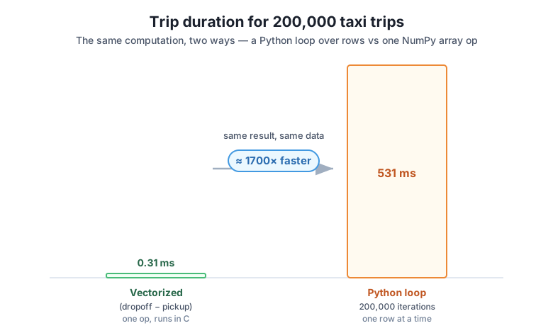
Speedup:         1709x faster

The Python loop spends about 531 milliseconds grinding through 200,000 iterations. The vectorized subtraction finishes the identical work in about 0.31 milliseconds — roughly 1,700 times faster. That is not a typo or a warm-cache fluke; the gap is the difference between running a loop in the Python interpreter and running it in compiled C, and it holds every time you re-run the block.

More vectorized ops your pipeline needs#

Duration is one derived column. A real pipeline builds many, and the same “operate on the whole array” habit produces all of them. Here are the three moves you’ll reach for constantly.

Element-wise arithmetic#

Any arithmetic between arrays (or between an array and a single number) happens element by element, in one pass. CityFlow wants an average-speed column, in miles per hour, from the trip distance and the duration you just computed. Speed is distance divided by time in hours — one expression over the whole array (guarding the handful of zero-duration trips so you never divide by zero):

distance = trips["trip_distance"].to_numpy()
moving = duration_min > 0                       # avoid divide-by-zero
speed_mph = np.zeros(len(trips))
speed_mph[moving] = distance[moving] / (duration_min[moving] / 60.0)

print("first 5 distances (mi): ", np.round(distance[:5], 2))
print("first 5 speeds (mph):   ", np.round(speed_mph[:5], 1))

first 5 distances (mi):  [17.14  2.49  1.84  3.6   0.04]
first 5 speeds (mph):    [32.2 14.1 16.2  7.2  1.5]

A 17-mile trip that took about 32 minutes averaged 32 mph — a highway airport run — while a short crawl through Manhattan traffic managed 1.5 mph. Every speed was computed at once, and speed_mph[moving] = ... even wrote the results back to only the rows that matter, again with no loop.

Comparisons and boolean masks#

A comparison on an array returns a boolean mask: an array of True/False, one per element. CityFlow flags unusually long trips — anything over an hour — for a data-quality check. The comparison is the flag column:

long_trip = duration_min > 60          # a boolean array, one flag per trip
print("dtype:", long_trip.dtype)
print("first 8 flags:", long_trip[:8])
print("trips over 60 min:", f"{long_trip.sum():,}")
print("share over 60 min:", f"{long_trip.mean() * 100:.2f}%")

dtype: bool
first 8 flags: [False False False False False False False False]
trips over 60 min: 2,012
share over 60 min: 1.01%

Two more idioms are hiding in that output. Summing a boolean array counts the True values (Python treats True as 1), so long_trip.sum() says 2,012 trips ran over an hour. Taking its mean gives the proportion that are True, so long_trip.mean() reports 1.01%. Count-how-many and what-share, both from one comparison and no loop.

np.where for a conditional column#

When you want a new column whose value depends on a condition — the vectorized cousin of an if/else — reach for np.where(condition, value_if_true, value_if_false). Nesting it handles more than two cases. Here CityFlow buckets every trip into a length band for the dashboard:

trip_band = np.where(duration_min <= 10, "quick",
             np.where(duration_min <= 30, "normal", "long"))

print("first 8 bands:", trip_band[:8])
labels, counts = np.unique(trip_band, return_counts=True)
for label, count in zip(labels, counts):
    print(f"  {label:6s}: {count:,}")

first 8 bands: ['long' 'normal' 'quick' 'normal' 'quick' 'quick' 'quick' 'normal']
  long  : 18,090
  normal: 98,373
  quick : 83,537

One np.where expression assigned all 200,000 labels in a single pass: about 83,500 quick hops of ten minutes or less, 98,000 normal trips, and 18,000 longer rides. The equivalent if/elif/else inside a Python loop would have produced the same buckets far more slowly and in three times the code.

The mental shift: think in whole arrays, not elements#

The techniques above share one habit worth naming, because it is the real lesson. When you have an array and a calculation, resist the instinct to loop over the elements. Instead ask: what is the single operation that produces the whole answer column at once? Subtract two columns. Multiply an array by a number. Compare a column to a threshold. Choose between labels with np.where. Each is one expression that NumPy pushes down into C and runs across every row in one tight pass.

This “think in whole arrays” mindset pays twice. The obvious dividend is speed — the roughly 1,700x you measured. The quieter one is clarity: duration_min = (dropoff - pickup) / np.timedelta64(1, "m") states the intent in a single readable line, while the loop that computes the same thing buries that intent under an index variable, a pre-allocated output array, and a range. Vectorized code is usually both the faster version and the one that reads like the formula it implements. When you find yourself writing for i in range(len(...)) over a NumPy array, treat it as a prompt to stop and look for the array operation you actually want.

Practice Exercises#

Exercise 1: Duration in seconds, and the longest trip#

Starting from the pickup and dropoff arrays, compute a vectorized duration_sec array (minutes won’t do here) by dividing the timedelta64 difference by one second. Print the mean duration in seconds and, using np.argmax, the length of the single longest trip in minutes. Do it with array operations only — no for loop.

Exercise 2: A tip-percentage column with a boolean summary#

Pull tip_amount and fare_amount out as arrays and build a vectorized tip_pct column: tip divided by fare, times 100, but only where fare_amount > 0 (use a boolean mask to protect against dividing by zero, exactly as the speed example did). Then make a boolean mask for “generous” trips where the tip is at least 25% of the fare, and print both how many such trips there are and what share of all trips they make up.

Exercise 3: Bucket trips by distance with np.where#

Using the trip_distance array, create a distance_band column with three labels: "short" for trips of 2 miles or less, "medium" for more than 2 up to 10 miles, and "long" for anything over 10. Print the count in each band with np.unique(..., return_counts=True). Then, as a one-line check, print what fraction of trips are "short" using a boolean mask rather than the counts.

Summary#

You replaced a Python loop with a single NumPy array operation and measured what it bought you. Computing trip duration in minutes for 200,000 real taxi trips took about 531 ms as a for loop and about 0.31 ms as a vectorized datetime64 subtraction — roughly a 1,700x speedup for a byte-for-byte identical result, confirmed with np.allclose. You then built the other columns a pipeline needs the same way: element-wise arithmetic for speed in mph, boolean masks to flag and count trips over an hour, and np.where to bucket every trip into a length band — each one expression, no loop.

Key Concepts#

• Vectorization expresses a whole-array computation as one NumPy operation that runs in compiled C, replacing a Python loop and its per-element interpreter overhead.
• Date math is vectorized too. Subtracting two datetime64 arrays yields a timedelta64 array; dividing by np.timedelta64(1, "m") converts a whole duration column to minutes.
• The speedup is measurable and large. On 200,000 rows the loop took ~531 ms and the array op ~0.31 ms; the exact multiple varies by machine but stays in the hundreds-to-thousands.
• Comparisons make boolean masks. A condition like duration_min > 60 returns a True/False array; .sum() counts the Trues and .mean() gives their share.
• np.where(cond, a, b) is the vectorized if/else, and nesting it handles more than two cases — a conditional column with no loop.
• Think in whole arrays. Vectorized code is usually both faster and clearer than the equivalent loop, because it reads like the formula it implements.

Why This Matters#

Every derived column in CityFlow’s pipeline — duration, speed, tip percentage, quality flags, length bands — is a calculation over millions of rows, and how you express that calculation decides whether the pipeline runs in milliseconds or grinds for minutes. Data engineers reach for vectorized operations by default not because loops are wrong but because, at scale, a loop in the Python interpreter is the single most common reason a pipeline is needlessly slow. The 1,700x you measured on one small column is the everyday payoff of a habit: when you have an array and a calculation, find the one array operation that does it. That habit is what lets the same code that handled 200,000 rows keep up when the data grows to millions.

Continue Building Your Skills#

You can now turn a loop into a single array operation and prove the speedup with a number. Every example so far, though, combined arrays of the same length — dropoff minus pickup, distance over duration. In Lesson 4 you’ll meet broadcasting: NumPy’s rules for combining arrays of different shapes without writing a loop or copying data, so you can do things like subtract a per-zone average from every trip, or scale a whole column by a single factor, cleanly and in one pass. It is the last core NumPy skill before the module’s guided project puts all of it — dtypes, vectorization, and broadcasting — to work computing CityFlow’s real per-trip metrics at once.