Title here
Summary here
In Lesson 3 you replaced Python loops with vectorized array math and watched the runtime collapse — but every example combined arrays of the same shape: distance times distance, fare minus fare. Real CityFlow work is rarely that tidy. You want to multiply a whole trip_distance column by a single conversion factor, or subtract one number per column from a two-dimensional block of trips. The shapes don’t match, and yet you still want clean, loop-free, whole-array math.
That is exactly what broadcasting is for. Broadcasting is the set of rules NumPy uses to stretch a smaller array across a larger one so that element-wise operations line up — automatically, and without ever building the big intermediate copy a loop would. In this lesson you’ll use it three ways on the real taxi sample: scale trip_distance from miles to kilometres with a single scalar, compute a real fare_per_mile for every trip, and center four money columns by subtracting their per-column means. Along the way you’ll see the memory stay tiny (no copy is made), and you’ll learn to read the one error broadcasting throws so a shape mismatch never stalls you for long. Every number below was measured on the 200,000-row NYC taxi sample your team develops against.
By the end of this lesson, you will be able to:
trip_distance miles to kilometresfare_per_mile as an element-wise array-by-array division(k,) vector of per-column means from an (N, k) array to center it, and confirm NumPy does not copy the vectorValueError: operands could not be broadcast together message and fix the shape mismatchYou only need numpy and pandas. Let’s stretch some arrays.
When you write a * b with two NumPy arrays of the same shape, NumPy pairs up matching elements and operates on each pair. Broadcasting answers a different question: what should happen when the shapes are not the same? Instead of refusing, NumPy tries to stretch the smaller array so its shape matches the larger one, then does the element-wise operation as usual. The stretch is virtual — NumPy reuses the small array’s values in place rather than physically building a bigger array — so you get the convenience of “repeat this value everywhere” with none of the memory cost.
The simplest case is a scalar. Load the sample and multiply the whole distance column by one number:
import warnings
warnings.filterwarnings("ignore")
import numpy as np
import pandas as pd

taxi = pd.read_csv("https://datatweets.com/datasets/nyc-taxi/yellow_tripdata_sample.csv")
distance_miles = taxi["trip_distance"].to_numpy()

# One scalar (1.60934) broadcasts across all 200,000 elements
distance_km = distance_miles * 1.60934

print("array shape:", distance_miles.shape)
print("first 5 miles:", np.round(distance_miles[:5], 2))
print("first 5 km:   ", np.round(distance_km[:5], 2))
array shape: (200000,)
first 5 miles: [17.14 2.49 1.84 3.6 0.04]
first 5 km: [27.58 4.01 2.96 5.79 0.06]The scalar 1.60934 has no shape at all, yet NumPy applied it to all 200,000 distances at once. Conceptually it was stretched into an array of 200,000 copies of 1.60934; in reality NumPy just multiplied each element by the one value it already had. A 17.14-mile ride becomes a 27.58-kilometre ride, and you wrote no loop. This is the mental model to carry into everything that follows: broadcasting = stretch the small operand to fit the big one, without materialising the copies.
Scalars are the friendly case. To combine two real arrays of different shapes, NumPy follows one precise rule, and it is worth memorizing because it explains every success and every error you will ever hit.
Compare the two shapes element by element, starting from the right (the last axis) and moving left. For each pair of dimensions, the operation is allowed only if they are equal, or one of them is 1. A missing dimension on the shorter shape is treated as 1. Wherever a dimension is 1 (or missing), that array is stretched along that axis to match the other.
A few worked shapes make the rule concrete:
| Left shape | Right shape | Aligned right-to-left | Result | Why |
|---|---|---|---|---|
(200000,) | () (scalar) | 200000 vs 1 | (200000,) | scalar stretches to every element |
(200000, 4) | (4,) | 4 vs 4, then 200000 vs 1 | (200000, 4) | the 4-vector repeats down all rows |
(200000, 4) | (200000, 1) | 4 vs 1, then 200000 vs 200000 | (200000, 4) | the column repeats across all 4 columns |
(200000, 4) | (3,) | 4 vs 3 | error | last axes 4 and 3 are unequal and neither is 1 |
Notice the pattern in row two: a (4,) vector lined up against a (200000, 4) array matches on the last axis (4 = 4), and its missing first axis is treated as 1, so it stretches across all 200,000 rows. That single row of the table is the engine behind column-wise centering, which you’ll build in a moment. Row four is the failure case — we’ll trigger it on purpose later so you know the message on sight.
Right-to-left is the whole trick
Almost every broadcasting surprise comes from forgetting that NumPy aligns shapes from the last axis backward, not the first. A (4,) vector broadcasts naturally against the columns of an (N, 4) array because 4 is the trailing dimension of both. If you instead wanted to broadcast one value per row, you would need a column-shaped (N, 1) array — same numbers, different shape — so the 1 lands on the trailing axis. Getting the shape right is 90% of broadcasting.
Scaling by a scalar is broadcasting with the smallest possible operand. The other everyday case is two full arrays of the same length combined element by element — pure vectorization, no stretching needed — which is how you turn two raw columns into a derived metric. CityFlow’s dashboard wants fare_per_mile: for each trip, fare_amount divided by trip_distance.
There is one real-world snag. Some trips have a trip_distance of 0.00 (the meter recorded no distance), and dividing by zero is undefined. Filter those out first with a boolean mask, then divide the two aligned arrays:
import warnings
warnings.filterwarnings("ignore")
import numpy as np
import pandas as pd

taxi = pd.read_csv("https://datatweets.com/datasets/nyc-taxi/yellow_tripdata_sample.csv")
fare = taxi["fare_amount"].to_numpy()
distance = taxi["trip_distance"].to_numpy()

valid = distance > 0                      # boolean mask, shape (200000,)
fare_per_mile = fare[valid] / distance[valid]   # element-wise, same shape

print("trips kept:", valid.sum(), "of", len(distance))
print("first 5 fare/mile:", np.round(fare_per_mile[:5], 2))
print("median fare/mile: %.2f" % np.median(fare_per_mile))
print("mean fare/mile:   %.2f" % np.mean(fare_per_mile))
trips kept: 196020 of 200000
first 5 fare/mile: [ 4.08 5.42 5.43 6.47 92.5 ]
median fare/mile: 7.16
mean fare/mile: 10.53Both fare[valid] and distance[valid] have the same shape — 196,020 elements — so this is element-wise division with no stretching: trip i’s fare pairs with trip i’s distance. The result is instantly informative. A typical NYC ride costs about $7.16 per mile (the median), but the mean is a much higher $10.53. That gap is the fingerprint of dirty data: look at the fifth kept trip, $92.50 per mile. A tiny 0.04-mile crawl with a normal minimum fare produces an enormous per-mile rate, and a handful of those outliers drag the average up while the median shrugs them off. Broadcasting and vectorization made the calculation trivial; noticing the median/mean split is the data-engineering judgment on top.
Why mask before dividing, not after
You could divide first and clean up the inf and nan values afterward, but masking first is cleaner and faster: NumPy never computes the undefined values at all, so no warnings are raised and no bad numbers sneak into your medians. The mask distance > 0 is itself a broadcast — a scalar 0 compared against all 200,000 distances — producing the boolean array you index with. Broadcasting shows up even in the filtering step.
Now the case broadcasting was really built for. A common preprocessing step before scaling, clustering, or feeding a model is centering: subtract each column’s mean so every column is expressed as a deviation from its own average. With a loop you would iterate column by column; with broadcasting it is a single subtraction.
Stack four numeric columns into one (200000, 4) array, compute the four column means (a (4,) vector), and subtract:
import warnings
warnings.filterwarnings("ignore")
import numpy as np
import pandas as pd

taxi = pd.read_csv("https://datatweets.com/datasets/nyc-taxi/yellow_tripdata_sample.csv")

cols = ["trip_distance", "fare_amount", "tip_amount", "total_amount"]
M = taxi[cols].to_numpy()          # shape (200000, 4)
col_means = M.mean(axis=0)         # shape (4,) — one mean per column

centered = M - col_means           # (200000, 4) - (4,)  broadcasts

print("M shape:        ", M.shape)
print("col_means shape:", col_means.shape)
print("col_means:      ", np.round(col_means, 2))
print("centered shape: ", centered.shape)
print("new column means:", np.round(centered.mean(axis=0), 10))
M shape: (200000, 4)
col_means shape: (4,)
col_means: [ 3.58 18.11 3.33 26.72]
centered shape: (200000, 4)
new column means: [-0. 0. -0. 0.]Read the shapes against the rule: (200000, 4) minus (4,). Aligning right-to-left, the last axes are 4 and 4 (equal — good), and the vector’s missing first axis is treated as 1, so it stretches down all 200,000 rows. The average trip in the sample is 3.58 miles, $18.11 fare, $3.33 tip, $26.72 total — and after subtracting those, each column’s new mean is zero (the -0. is floating-point rounding of a value like -0.0000000001). One line centered 800,000 numbers.
Look at what happened to the very first trip:
import warnings
warnings.filterwarnings("ignore")
import numpy as np
import pandas as pd

taxi = pd.read_csv("https://datatweets.com/datasets/nyc-taxi/yellow_tripdata_sample.csv")
cols = ["trip_distance", "fare_amount", "tip_amount", "total_amount"]
M = taxi[cols].to_numpy()
centered = M - M.mean(axis=0)

print("row 0 raw:     ", np.round(M[0], 2))
print("row 0 centered:", np.round(centered[0], 2))
row 0 raw: [17.14 70. 8.27 90.96]
row 0 centered: [13.56 51.89 4.94 64.24]That first trip was a long, expensive one: 17.14 miles, $70.00 fare. Centered, it reads +13.56 miles, +51.89 dollars — “well above average on every measure.” The figure below shows the whole operation: the (4,) mean vector conceptually repeated down every row of M, producing the centered result of the same shape.
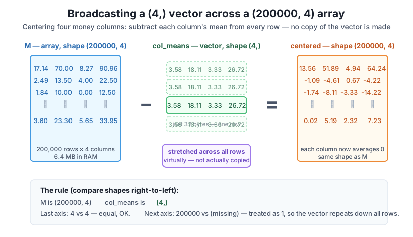
(N, 4) array by subtracting a (4,) mean vector. The rule aligns shapes right-to-left: the trailing axis matches (4 = 4), and the vector's missing leading axis is treated as 1, so the same 32-byte mean vector is stretched down all 200,000 rows — virtually, never physically copied. The result keeps the original (200000, 4) shape, and each centered column now averages zero. This one subtraction replaces a Python loop over columns.The whole promise of broadcasting is that the small array is stretched virtually — NumPy never builds the big repeated copy. It’s worth proving to yourself, because the alternative (physically repeating the vector) is what a naive loop-free approach might do, and it wastes memory. The manual way to line up shapes is np.tile, which really does build the full (200000, 4) block:
import warnings
warnings.filterwarnings("ignore")
import numpy as np
import pandas as pd

taxi = pd.read_csv("https://datatweets.com/datasets/nyc-taxi/yellow_tripdata_sample.csv")
cols = ["trip_distance", "fare_amount", "tip_amount", "total_amount"]
M = taxi[cols].to_numpy()
col_means = M.mean(axis=0)

tiled = np.tile(col_means, (M.shape[0], 1))   # physically repeat into (200000, 4)

print("col_means shape:", col_means.shape, "->", col_means.nbytes, "bytes")
print("tiled shape:    ", tiled.shape, "->", tiled.nbytes, "bytes",
      "(%.1f MB)" % (tiled.nbytes / 1024 / 1024))
print("same result?", np.array_equal(M - col_means, M - tiled))
col_means shape: (4,) -> 32 bytes
tiled shape: (200000, 4) -> 6400000 bytes (6.1 MB)
same result? TrueThe broadcast operand is 32 bytes. The physically tiled version is 6.1 MB — 200,000 times larger — and yet both produce the identical centered array. Broadcasting gave you the tiled result without ever paying for the 6.1 MB copy. On the 200,000-row sample that saving is modest; on the full 2.96-million-row month it is the difference between a subtraction that fits comfortably in RAM and one that needlessly duplicates a chunk of your working memory. When you can broadcast, never tile.
Broadcasting fails loudly and consistently, so learning to read the one error it raises pays off every time a shape is wrong. Suppose you try to center M with a mean vector of the wrong length — three values instead of four (perhaps you forgot a column):
import warnings
warnings.filterwarnings("ignore")
import numpy as np
import pandas as pd

taxi = pd.read_csv("https://datatweets.com/datasets/nyc-taxi/yellow_tripdata_sample.csv")
cols = ["trip_distance", "fare_amount", "tip_amount", "total_amount"]
M = taxi[cols].to_numpy()                 # shape (200000, 4)

wrong = np.array([1.0, 2.0, 3.0])         # length 3, not 4

try:
    result = M - wrong
except ValueError as e:
    print("ValueError:", e)
ValueError: operands could not be broadcast together with shapes (200000,4) (3,) The message hands you everything you need. It names the operation (“could not be broadcast together”) and prints both shapes: (200000,4) and (3,). Apply the rule yourself, right-to-left: the trailing axes are 4 and 3 — not equal, and neither is 1 — so broadcasting is impossible, and NumPy stops before computing anything. The fix is always to make the trailing dimensions agree: here, the mean vector must have length 4 to match M’s four columns. Whenever you see this error, read off the two printed shapes, align them from the right, and find the axis where they are neither equal nor 1 — that pair is your bug.
A fast debugging habit
Before combining two arrays whose shapes you’re unsure of, print a.shape and b.shape and mentally align them from the right. If every trailing pair is equal-or-one, it will broadcast; the first pair that is neither tells you exactly which axis to reshape. Reaching for .shape first turns “why won’t this work” into a five-second check.
Exercise 1 — Kilometres and a speed sanity check. Load the taxi sample, pull trip_distance into a NumPy array, and broadcast the scalar 1.60934 to produce distance_km. Then print the mean of distance_miles and the mean of distance_km, and confirm the km mean is about 1.609 times the miles mean.
Hint
distance_km = taxi["trip_distance"].to_numpy() * 1.60934. Use np.mean(...) (or .mean()) on each array. The ratio distance_km.mean() / distance_miles.mean() should print very close to 1.60934 — because multiplying every element by a constant multiplies the mean by the same constant.
Exercise 2 — Tip rate, element-wise. Compute tip_rate = tip_amount / total_amount for every trip where total_amount is greater than zero, using a boolean mask exactly like the fare_per_mile example. Print how many trips you kept, and the median tip rate as a percentage.
Hint
Build valid = taxi["total_amount"].to_numpy() > 0, then divide tip[valid] / total[valid] where both are NumPy arrays. Multiply the median by 100 for a percentage: np.median(tip_rate) * 100. Masking first avoids any divide-by-zero on trips with a zero total.
Exercise 3 — Broadcast per row instead of per column. Take the same (200000, 4) array M, and this time divide every value by that trip’s total_amount so each row is expressed as a fraction of its total. You’ll need the totals shaped as a column, (200000, 1), not a flat (200000,). Confirm the result has shape (200000, 4), then explain in one sentence why the reshape was necessary.
Hint
totals = M[:, 3].reshape(-1, 1) gives shape (200000, 1); then M / totals broadcasts the single column across all four columns (last axes 4 vs 1). If you used the flat (200000,) shape instead, NumPy would try to align 200000 against the trailing axis 4 and raise the broadcasting error — the reshape puts the 1 on the trailing axis so it stretches across columns, not down rows.
You learned how NumPy combines arrays of different shapes without loops or copies. Broadcasting stretches the smaller operand to match the larger one and then does the element-wise operation — virtually, so no big intermediate array is built. The rule is a single sentence: compare shapes right-to-left, and each pair of dimensions must be equal or one of them must be 1. You broadcast a scalar to convert trip_distance from miles to kilometres (17.14 miles becomes 27.58 km), divided two aligned arrays to get a real fare_per_mile (median $7.16, mean $10.53 — the gap exposing short-trip outliers like $92.50/mile), and subtracted a (4,) mean vector from a (200000, 4) array to center four money columns in one line, driving every column’s mean to zero. You proved the mean vector was 32 bytes while a physically tiled copy would have been 6.1 MB, and you read the ValueError: operands could not be broadcast together with shapes (200000,4) (3,) message and traced it to the mismatched trailing axis.
miles * 1.60934.(N, k) minus (k,) — a per-column vector broadcasts down all rows because the trailing axes match; this is how you center or scale columns in one operation.np.tile), which is why it is both fast and memory-lean.operands could not be broadcast together with shapes ... prints both shapes; align them right-to-left and the first pair that is neither equal nor 1 is the bug.CityFlow’s pipeline is full of “one value applied to many” and “one value per column” operations: unit conversions, per-trip rates, normalising a block of columns before a model sees it. Broadcasting lets you express all of them as short, readable, whole-array math that runs at C speed and doesn’t balloon memory — the two constraints this entire course is about. Just as important, understanding the shape rule turns the one error broadcasting raises from a mystery into a two-line fix, so a shape mismatch costs you seconds instead of an afternoon. Every higher-level tool you’ll meet later, pandas included, broadcasts under the hood; knowing the rule means you can predict and debug their behaviour instead of guessing.
You can now combine arrays of any compatible shapes without loops or copies, and you’ve centered real taxi columns with a single broadcast subtraction. Lesson 5, the module’s guided project Compute Trip Metrics on the Taxi Data, puts everything from this module together: you’ll load the taxi columns as NumPy arrays, then use vectorization and broadcasting to derive a full set of per-trip metrics — trip duration, average speed, fare_per_mile, and tip rate — memory-lean and loop-free, exactly as CityFlow’s dashboard pipeline needs them. Bring the shape rule and the miles-to-km, fare-per-mile, and centering patterns from this lesson; you’ll reach for every one of them.
Keep DATATWEETS free. Help fund practical data, AI, and engineering lessons for learners worldwide.

