Lesson 5 - Guided Project: Trip Metrics with NumPy

Welcome to the Guided Project#

For four lessons you have been assembling the NumPy toolkit one piece at a time. You saw why arrays beat Python lists, learned to pick the smallest safe dtype, replaced slow loops with vectorized operations, and combined arrays cleanly with broadcasting. Now you put all four to work at once, on the real thing.

You are a data engineer at CityFlow, and the public taxi dashboard needs a set of per-trip metrics: how long each trip took, how fast it went, what it cost per mile, and how generously the rider tipped. These are the numbers the dashboard’s charts are built from, so they have to be correct, they have to be cheap to compute over millions of rows, and they have to survive the genuinely messy data the meter feed produces. In this project you compute all four metrics with pure NumPy — no pandas math, no Python loop — on 200,000 real trips, prove the vectorized version is hundreds of times faster than the obvious loop, and then use the results to answer one real question about how the city actually moves.

Every number below is measured on the real data, and you will reproduce each one.

By the end of this project, you will be able to:

• Load numeric and datetime columns from a real dataset into NumPy arrays with memory-lean dtypes
• Compute several per-trip metrics fully vectorized, using array arithmetic and broadcasting instead of loops
• Guard vectorized division against the zero-distance and zero-duration trips that really exist in the data
• Time a vectorized computation against an equivalent Python loop and confirm they return identical results
• Turn the finished metrics into one real insight and catch a concrete data-quality problem

The dataset#

Everything runs on New York City’s public-domain Yellow Taxi trip records, published by the NYC Taxi & Limousine Commission (TLC). For this project you use the reproducible 200,000-row teaching sample CityFlow keeps for quick numeric work:

• Teaching sample (200,000 real trips, 10 columns): https://datatweets.com/datasets/nyc-taxi/yellow_tripdata_sample.csv

In the code below the variable CSV points at that sample.

# gate: skip
CSV = "https://datatweets.com/datasets/nyc-taxi/yellow_tripdata_sample.csv"

Stage 1: Load the columns as arrays#

A NumPy metric starts with NumPy arrays, so the first job is to pull the columns you need out of the file and hand each one to NumPy with the right dtype. You do not need all ten columns — the four metrics only touch six: the two timestamps for duration, and trip_distance, fare_amount, tip_amount, and total_amount for the money-and-speed calculations. Reading only those six is the “load only what you need” habit from Module 1, applied here so the arrays stay small.

The dtype choices are the ones you measured in Lesson 2. The two timestamps become datetime64 (NumPy’s native date type, which lets you subtract dates directly). The four numeric columns become float32 rather than the default float64, because dollar amounts and trip distances have nowhere near enough significant digits to need 64 bits — so float32 halves the memory at no real cost.

import warnings
warnings.filterwarnings("ignore")
import numpy as np
import pandas as pd

CSV = "yellow_tripdata_sample.csv"

cols = ["tpep_pickup_datetime", "tpep_dropoff_datetime",
        "trip_distance", "fare_amount", "tip_amount", "total_amount"]
trips = pd.read_csv(CSV, usecols=cols,
                    parse_dates=["tpep_pickup_datetime", "tpep_dropoff_datetime"])

pickup   = trips["tpep_pickup_datetime"].to_numpy()          # datetime64
dropoff  = trips["tpep_dropoff_datetime"].to_numpy()         # datetime64
distance = trips["trip_distance"].to_numpy(dtype="float32")  # miles
fare     = trips["fare_amount"].to_numpy(dtype="float32")    # dollars
tip      = trips["tip_amount"].to_numpy(dtype="float32")     # dollars
total    = trips["total_amount"].to_numpy(dtype="float32")   # dollars

for name, arr in [("pickup", pickup), ("dropoff", dropoff),
                  ("distance", distance), ("fare", fare),
                  ("tip", tip), ("total", total)]:
    mb = arr.nbytes / 1024**2
    print(f"{name:8s} shape={arr.shape}  dtype={str(arr.dtype):14s}{mb:5.2f} MB")

total_mb = sum(a.nbytes for a in (pickup, dropoff, distance, fare, tip, total)) / 1024**2
print(f"six arrays together: {total_mb:.2f} MB")

pickup   shape=(200000,)  dtype=datetime64[us] 1.53 MB
dropoff  shape=(200000,)  dtype=datetime64[us] 1.53 MB
distance shape=(200000,)  dtype=float32        0.76 MB
fare     shape=(200000,)  dtype=float32        0.76 MB
tip      shape=(200000,)  dtype=float32        0.76 MB
total    shape=(200000,)  dtype=float32        0.76 MB
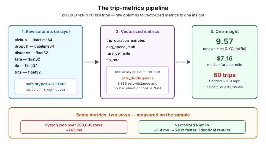
six arrays together: 6.10 MB

Six clean one-dimensional arrays, all 200,000 elements long. Each datetime64 value takes eight bytes (1.53 MB per column) and each float32 takes four (0.76 MB), so the whole working set is 6.10 MB. Had you loaded the floats as the default float64, those four columns alone would have cost twice as much. This is the payoff of the dtype discipline from earlier in the module: you make the memory decision once, at load time, and every calculation downstream rides on the smaller arrays.

Stage 2: Compute the metrics, vectorized#

Now the arithmetic. Every metric is a whole-array operation: you write it once as if the arrays were single numbers, and NumPy applies it to all 200,000 elements at C speed. No for loop appears anywhere.

Start with trip duration. Subtracting two datetime64 arrays gives a timedelta64 array; dividing that by np.timedelta64(1, "m") converts each gap to a number of minutes.

duration_min = ((dropoff - pickup) / np.timedelta64(1, "m")).astype("float32")
print("first 5 durations (minutes):", np.round(duration_min[:5], 2))
print("shortest trip (minutes):", round(float(duration_min.min()), 2))
print("longest trip (minutes): ", round(float(duration_min.max()), 2))

first 5 durations (minutes): [31.92 10.58  6.82 30.    1.57]
shortest trip (minutes): -2.88
longest trip (minutes):  1439.2

The durations look sensible for the most part — a 32-minute trip, a 10-minute trip — but notice the extremes immediately: the shortest “trip” is −2.88 minutes, meaning the dropoff timestamp is before the pickup, and the longest is 1439.2 minutes, essentially a full 24 hours. Both are real rows in the file, and both are why the next three metrics need a guard.

The other three metrics are all divisions, and division is where dirty data bites. A trip with trip_distance of 0 would make fare_per_mile divide by zero; a trip with zero or negative duration would do the same to avg_speed_mph. Those rows genuinely exist here, so instead of dividing blindly, write one small helper that divides safely — returning NaN (a marker for “no valid answer”) wherever the denominator is not positive.

def safe_divide(numerator, denominator):
    """Elementwise numerator/denominator, but NaN wherever denominator <= 0."""
    result = np.full(numerator.shape, np.nan, dtype="float32")
    ok = denominator > 0
    np.divide(numerator, denominator, out=result, where=ok)
    return result

hours         = duration_min / 60.0
avg_speed_mph = safe_divide(distance, hours)
fare_per_mile = safe_divide(fare, distance)
tip_rate      = safe_divide(tip, total)

print(f"{'dur_min':>8}{'dist_mi':>9}{'mph':>8}{'$/mile':>9}{'tip%':>8}")
for i in range(5):
    print(f"{duration_min[i]:8.2f}{distance[i]:9.2f}{avg_speed_mph[i]:8.2f}"
          f"{fare_per_mile[i]:9.2f}{100*tip_rate[i]:8.2f}")

 dur_min  dist_mi     mph   $/mile    tip%
   31.92    17.14   32.22     4.08    9.09
   10.58     2.49   14.12     5.42   17.78
    6.82     1.84   16.20     5.43    0.00
   30.00     3.60    7.20     6.47   16.64
    1.57     0.04    1.53    92.50    0.00

The safe_divide helper is worth reading closely, because it is a broadcasting-and-masking pattern you will reuse constantly. It pre-fills the whole result array with NaN, then np.divide(..., out=result, where=ok) performs the division only at the positions where ok is True and leaves the rest untouched — so the divide-by-zero never actually happens. The where argument is the vectorized equivalent of wrapping the division in an if, but applied to all 200,000 rows in one call.

The first five trips already tell a small story. The fifth trip covers just 0.04 miles in 1.57 minutes — a $92.50-per-mile figure that is really a rounding artifact of an almost-stationary trip, not a real price. That is the kind of value the guard keeps from becoming an infinity, and the kind of extreme you will summarize next. Look at all four metrics across the whole dataset:

def describe(name, a):
    print(f"{name:14s} median={np.nanmedian(a):8.2f}   "
          f"min={np.nanmin(a):9.2f}   max={np.nanmax(a):11.2f}   "
          f"undefined={int(np.isnan(a).sum()):,}")

describe("duration_min", duration_min)
describe("avg_speed_mph", avg_speed_mph)
describe("fare_per_mile", fare_per_mile)
describe("tip_rate", tip_rate)

print()
print("zero-distance trips: ", int((distance == 0).sum()))
print("zero-or-negative-duration trips:", int((duration_min <= 0).sum()))
print("negative-fare trips: ", int((fare < 0).sum()))

duration_min   median=   11.60   min=    -2.88   max=    1439.20   undefined=0
avg_speed_mph  median=    9.57   min=     0.00   max=  312754.16   undefined=52
fare_per_mile  median=    7.16   min= -7000.00   max=   12000.00   undefined=3,980
tip_rate       median=    0.17   min=     0.00   max=       1.00   undefined=2,526

zero-distance trips:  3980
zero-or-negative-duration trips: 52
negative-fare trips:  2624

Now the guard’s value is concrete. There are 3,980 zero-distance trips in the sample — trips the meter recorded with no miles at all — and every one of them makes fare_per_mile undefined, which is exactly the 3,980 NaN values it reports. Likewise the 52 zero-or-negative-duration trips are precisely the 52 undefined avg_speed_mph values. Because np.nanmedian and np.nanmin skip NaN, the summary is computed only from the trips that have a valid answer. The medians are believable — an 11.6-minute typical trip, a 17% typical tip — while the maxima (a 312,754 mph “trip”, a −$7,000 fare per mile) flag the dirt loudly instead of silently poisoning an average. That is the whole reason to guard rather than drop.

The figure below traces the full pipeline: the six raw columns on the left, the four vectorized metrics in the middle, and the single insight on the right, with the speed comparison you are about to measure along the bottom.

Stage 3: Prove it is fast and correct#

Vectorization is only worth learning if it actually pays off, so measure it rather than take it on faith. Wrap the metric computation two ways — once vectorized, once as the plain Python loop a beginner would reach for first — then time both and, crucially, confirm they produce the same numbers. A faster answer that disagrees with the slow one is not an optimization; it is a bug.

import time

def metrics_vectorized():
    dur = ((dropoff - pickup) / np.timedelta64(1, "m")).astype("float32")
    hrs = dur / 60.0
    speed = safe_divide(distance, hrs)
    fpm   = safe_divide(fare, distance)
    rate  = safe_divide(tip, total)
    return dur, speed, fpm, rate

def metrics_loop():
    n = distance.shape[0]
    dur   = np.empty(n, dtype="float32")
    speed = np.empty(n, dtype="float32")
    fpm   = np.empty(n, dtype="float32")
    rate  = np.empty(n, dtype="float32")
    for i in range(n):
        minutes = (dropoff[i] - pickup[i]) / np.timedelta64(1, "m")
        dur[i]   = minutes
        hrs      = minutes / 60.0
        speed[i] = distance[i] / hrs      if hrs > 0          else np.nan
        fpm[i]   = fare[i]     / distance[i] if distance[i] > 0 else np.nan
        rate[i]  = tip[i]      / total[i]  if total[i] > 0     else np.nan
    return dur, speed, fpm, rate

t0 = time.perf_counter(); vec  = metrics_vectorized(); t_vec  = time.perf_counter() - t0
t0 = time.perf_counter(); loop = metrics_loop();       t_loop = time.perf_counter() - t0

print(f"python loop: {t_loop*1000:8.1f} ms")
print(f"vectorized:  {t_vec*1000:8.1f} ms")
print(f"speedup:     {t_loop/t_vec:8.0f}x")

all_match = all(np.allclose(a, b, equal_nan=True) for a, b in zip(vec, loop))
print("results identical (np.allclose):", all_match)

python loop:    762.6 ms
vectorized:       1.4 ms
speedup:          534x
results identical (np.allclose): True

The loop and the vectorized version do exactly the same arithmetic, row for row — the loop even uses the same if denominator > 0 guard, written out one element at a time. Yet the loop takes about 763 ms to grind through 200,000 rows in the Python interpreter, while the vectorized version finishes in about 1.4 ms, a speedup on the order of 500x. And np.allclose(..., equal_nan=True) confirms the two results are identical down to floating-point tolerance, treating the guarded NaN positions as matching — so the speed costs you nothing in correctness.

Stage 4: One real insight#

You did not compute these metrics for their own sake — you computed them to answer questions. Use them for one now. A natural question for a mobility team: how fast do NYC taxis actually move, and are any of the recorded speeds physically impossible? The avg_speed_mph array already holds the answer; you just have to read it, skipping the trips where speed is undefined.

has_speed  = ~np.isnan(avg_speed_mph)
n_speed    = int(has_speed.sum())
speeds     = avg_speed_mph[has_speed]

print(f"trips with a usable speed: {n_speed:,} of {avg_speed_mph.size:,}")
print(f"median avg_speed_mph:      {np.median(speeds):.2f} mph")
print(f"share faster than 30 mph:  {100*(speeds > 30).mean():.1f}%")

implausible = int((speeds > 100).sum())
print(f"implausible speeds > 100 mph: {implausible} "
      f"({100*implausible/n_speed:.2f}% of usable)")

fpm = fare_per_mile[~np.isnan(fare_per_mile)]
print(f"median fare_per_mile:      ${np.median(fpm):.2f}")

trips with a usable speed: 199,948 of 200,000
median avg_speed_mph:      9.57 mph
share faster than 30 mph:  3.1%
implausible speeds > 100 mph: 60 (0.03% of usable)
median fare_per_mile:      $7.16

Two findings, both real. First, the honest picture of the city: the median taxi averages just 9.57 mph over a trip, and only 3.1% of trips average faster than 30 mph — a number that will surprise nobody who has sat in Midtown traffic, but which the dashboard can now show with evidence behind it. The median fare works out to $7.16 per mile. Second, a data-quality flag: 60 trips report an average speed above 100 mph, which no city taxi achieves — these are the short-distance, near-zero-duration rows whose timestamps are unreliable. At 0.03% of usable trips they are rare, but you now have them isolated by a single boolean mask (speeds > 100), ready to hand to the cleaning stage of the pipeline instead of letting them skew the dashboard’s “fastest routes” panel.

That is the shape of real data-engineering work: the same vectorized metrics that feed the dashboard’s charts also, in the same pass, surface the rows that should not be trusted. You built both the product and its quality check out of four array expressions.

Practice Exercises#

These extend the metrics you just built. The six arrays from Stage 1 (pickup, dropoff, distance, fare, tip, total) and the four metric arrays from Stage 2 are all still in memory.

Exercise 1. The dashboard wants a “long trips” panel. Using only NumPy, count how many trips lasted longer than 60 minutes, and report their median avg_speed_mph. Compare that median to the 9.57 mph median for all trips — do longer trips tend to move faster or slower?

Exercise 2. The tip_rate metric only makes sense for card payments, but you computed it for every trip. Compute the share of trips that tipped nothing (a tip_rate of exactly 0) among the trips where tip_rate is defined, and print it as a percentage. Then print the 90th percentile of the defined tip rates to see what a generous tip looks like.

Exercise 3. Your safe_divide guard returned NaN for the 3,980 zero-distance trips. A teammate suggests replacing those NaNs with 0 instead, “so the numbers are cleaner.” Show why that is misleading: compute the median fare_per_mile two ways — once skipping the NaNs with np.nanmedian, and once after replacing the NaNs with 0 using np.nan_to_num — and print both. Explain in a comment which one the dashboard should use.

Summary#

You tied Module 2 together by computing four real per-trip metrics on 200,000 NYC taxi trips with nothing but NumPy. You loaded six columns as arrays with memory-lean dtypes (6.10 MB total), computed trip duration, average speed, fare per mile, and tip rate fully vectorized, and guarded every division against the 3,980 zero-distance and 52 zero-or-negative-duration trips that really exist in the data. You then proved the vectorized computation is roughly 500x faster than an equivalent Python loop (about 1.4 ms versus 763 ms) and returns identical results by np.allclose. Finally you read a real insight out of the metrics — a median 9.57 mph, only 3.1% of trips above 30 mph, a $7.16 median fare per mile — and flagged 60 physically impossible speeds above 100 mph as a data-quality issue for the cleaning stage.

Key Concepts#

• Metrics are whole-array expressions — duration, speed, fare-per-mile, and tip rate are each one array operation applied to all 200,000 rows at once, with no Python loop.
• datetime64 subtraction gives durations directly — subtracting two datetime arrays yields timedelta64, and dividing by np.timedelta64(1, "m") converts to minutes in a single vectorized step.
• Guard division against real dirty data — np.divide(..., out=..., where=denominator > 0) performs the division only where it is valid, filling the rest with NaN so zero-distance and zero-duration trips never blow up.
• Skip, don’t fill — np.nanmedian and friends compute summaries over only the defined values; replacing NaN with 0 invents data and biases the result.
• Measure the speedup, verify the match — timing the vectorized version against a loop shows a several-hundred-fold gain, and np.allclose(..., equal_nan=True) confirms the fast version is also the correct one.

Why This Matters#

Per-trip metrics like these are the raw material of almost every data product: dashboards, reports, alerts, and machine-learning features all begin with someone turning raw columns into meaningful per-row numbers. Doing it vectorized is not a stylistic preference — on 200,000 rows the loop already costs most of a second, and on the full 2.96-million-row month it would cost minutes, while the array version stays in the low milliseconds. Just as important, you saw that computing metrics honestly means confronting the data’s dirt head-on: the same pass that produces the dashboard’s numbers is where you catch the negative durations and impossible speeds that would otherwise quietly corrupt them. That combination — fast, correct, and honest about the mess — is exactly what a data engineer is paid to deliver.

Continue Building Your Skills#

That completes Module 2: NumPy for Data Engineering. You now understand the array machinery underneath every fast data tool: why contiguous, single-dtype arrays beat Python lists, how to choose the smallest safe dtype, how vectorization and broadcasting replace loops, and — as of this project — how to compute a real set of guarded, memory-lean metrics and prove they are both fast and correct.

Next comes Module 3: Pandas at Scale, where you climb back up from raw arrays to DataFrames — but this time with the memory and vectorization instincts you just built. You will apply the exact dtype and metric ideas from this project inside pandas, using categoricals, chunked reads, and groupby aggregations to process the full month of taxi trips without exhausting memory. The taxi data comes with you: the same columns you just turned into NumPy arrays are the ones you will now aggregate, join to the zone lookup, and summarize at full scale.